Processing 1D Bruker Data

Processing 1D Bruker Data

This example shows how nmrglue can be used to process and display one dimensional Bruker data.

Raw Bruker data from modern spectrometers contains a group delay artifact which must be removed during processing. There has been much speculation as to the origins of this artifact and many methods for removing the artifact have been suggested 1, 2, 3, 4, 5.

Nmrglue provides an algorithm for removing this artifact based on the protocol presented in "DMX DIGITAL FILTERS AND NON-BRUKER OFFLINE PROCESSING III" by W. M. Westler and F. Abildgaard. This method is available for use through nmrglue.fileio.bruker.remove_digital_filter. Nmrglue users can use this included function to remove the artifact or implement their own method if they are unsatisfied with the results.

In this example a 1D NMR spectrum of 1,3 diaminopropane is processed and plotted using nmrglue. The results can be compared with the spectrum produced from NMRPipe which provides a different artifact removal algorithm. Note that no apodization or baseline corrections are performed on these spectra.

Instructions

• Download the 1D proton spectrum of 1,3 diaminopropane and unpack in this directory. This raw data is available from the Madison Metabolomics Consortium Database as expnmr_00001_1.tar.

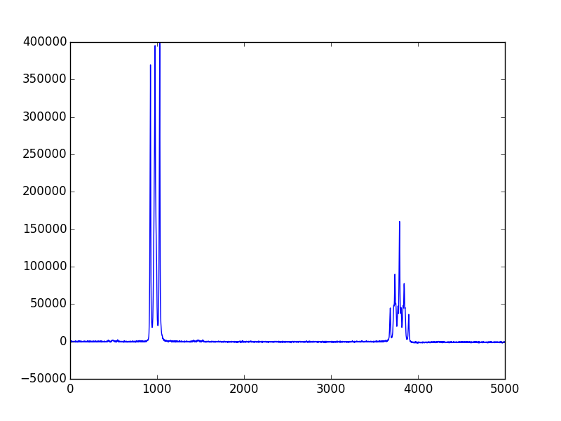
• Execute process_and_plot_nmrglue.py to process and plot the 1D spectrum. This creates the file figure_nmrglue.png.

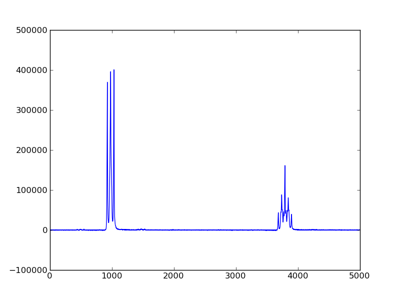
• Optionally, the data can be processed with NMRPipe using the script nmrpipe_proc.com. Then plot_nmrpipe.py can be used to plot the resulting spectrum. This creates the file figure_nmrpipe.png.

process_and_plot_nmrglue.py source code

#! /usr/bin/env python

import nmrglue as ng
import matplotlib.pyplot as plt

# read in the bruker formatted data
dic, data = ng.bruker.read('expnmr_00001_1')

# remove the digital filter
data = ng.bruker.remove_digital_filter(dic, data)

# process the spectrum
data = ng.proc_base.zf_size(data, 32768) # zero fill to 32768 points
data = ng.proc_base.fft(data) # Fourier transform
data = ng.proc_base.ps(data, p0=-88.0) # phase correction
data = ng.proc_base.di(data) # discard the imaginaries
data = ng.proc_base.rev(data) # reverse the data

fig = plt.figure()
ax = fig.add_subplot(111)
ax.plot(data[20000:25000])
fig.savefig('figure_nmrglue.png')

Output:

![1D Bruker data processed with nmrglue] (https://raw.github.com/jjhelmus/nmrglue/master/examples/bruker_data/figure_nmrglue.png)

[nmrpipe_proc.com source code] (https://raw.github.com/jjhelmus/nmrglue/blob/master/examples/bruker_data/nmrpipe_proc.com)

#!/bin/csh

bruk2pipe -in ./expnmr_00001_1/fid \
  -bad 0.0 -noaswap -DMX -decim 32 -dspfvs 12 -grpdly 0 \
  -xN 32768 \
  -xT 16384 \
  -xMODE DQD \
  -xSW 4807.692 \
  -xOBS 400.132 \
  -xCAR 4.697 \
  -xLAB 1H \
  -ndim 1 \
  -out ./test.fid -verb -ov

nmrPipe -in test.fid \
| nmrPipe -fn ZF -auto \
| nmrPipe -fn FT \
| nmrPipe -fn PS -p0 -22.0 -p1 0.0 -di \ 
  -out test.ft2 -verb -ov

[plot_nmrpipe.py source code] (https://raw.github.com/jjhelmus/nmrglue/blob/master/examples/bruker_data/plot_nmrpipe.py)

#! /usr/bin/env python

import nmrglue as ng
import matplotlib.pyplot as plt

# read in the data
dic, data = ng.pipe.read('test.ft2')

# plot the spectrum
fig = plt.figure()
ax = fig.add_subplot(111)
ax.plot(data[20000:25000])
fig.savefig('figure_nmrpipe.png')

Output:

![1D Bruker data processed with NMRPipe] (https://raw.github.com/jjhelmus/nmrglue/master/examples/bruker_data/figure_nmrpipe.png)

Note: a version of this example is also included in the nmrglue documentation