Reading Bruker processed files

Nmrglue has the ability to read spectral data from processed Bruker files which are typically found in the pdata directory.
This is accomplished using the nmrglue.bruker.read_pdata function.

For example, the 1D and 2D processed data of the antibacterial peptide capistruin (BMRB Entry 20014) can be [downloaded] (http://www.bmrb.wisc.edu/ftp/pub/bmrb/timedomain/bmr20014/timedomain_data/Capistruin.tar).

After extracting the Capistruin directory from this tar file, the following scripts can be executed in this directory to plot the spectra.

#! /usr/bin/env python

import nmrglue as ng
import matplotlib.pyplot as plt

dic, data = ng.bruker.read_pdata('10/pdata/1')

fig = plt.figure()
ax = fig.add_subplot(111)
ax.plot(data)
fig.savefig('proton_1d.png')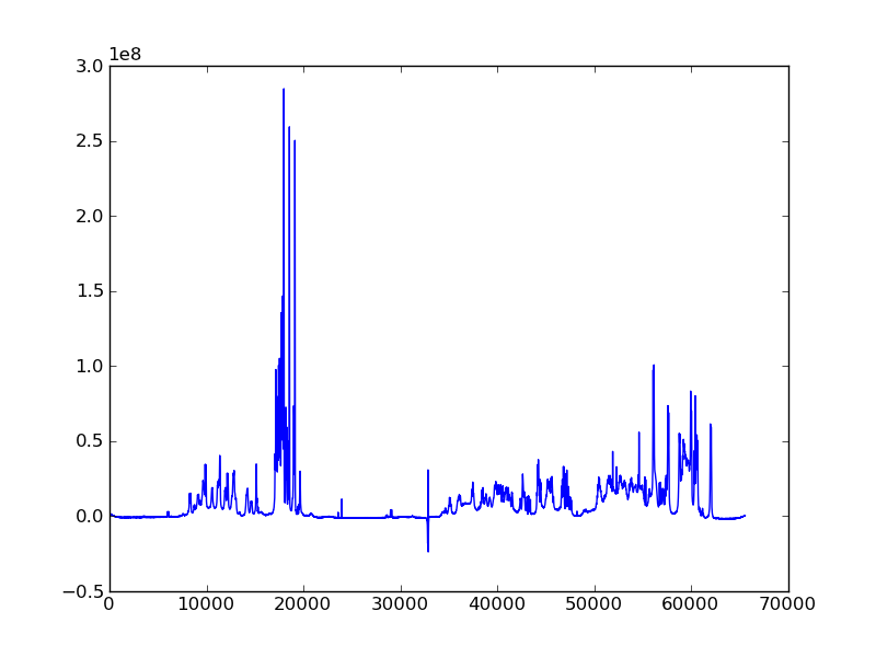

#! /usr/bin/env python

import numpy as np
import matplotlib.pyplot as plt
import nmrglue as ng

dic, data = ng.bruker.read_pdata('11/pdata/1')
cl = data.std() * 2 * 1.2 ** np.arange(10)
fig = plt.figure()
ax = fig.add_subplot(111)
ax.contour(data, cl, colors='blue')
fig.savefig('cosy_2d.png')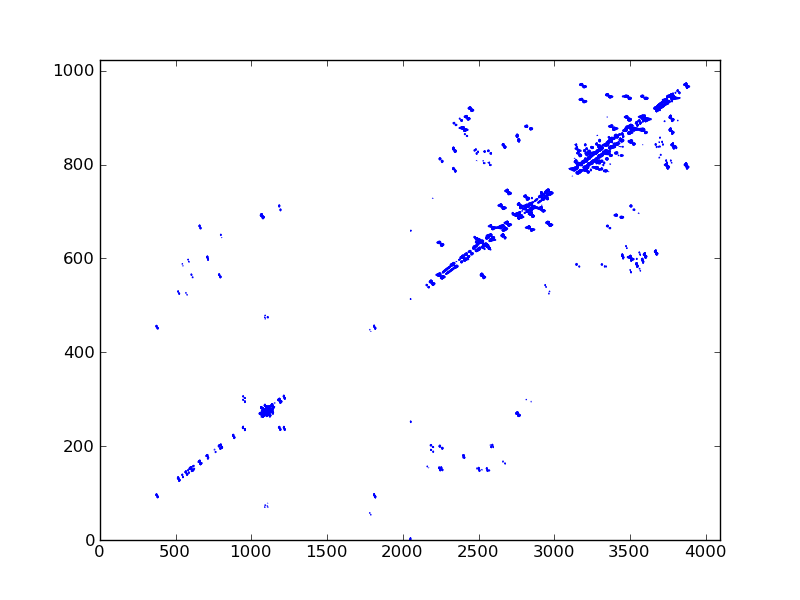

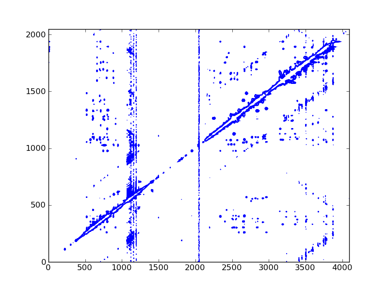
#! /usr/bin/env python

import numpy as np
import matplotlib.pyplot as plt
import nmrglue as ng

dic, data = ng.bruker.read_pdata('12/pdata/1')
cl = data.std() * 2 * 1.2 ** np.arange(10)
fig = plt.figure()
ax = fig.add_subplot(111)
ax.contour(data, cl, colors='blue')
fig.savefig('tocsy_2d.png')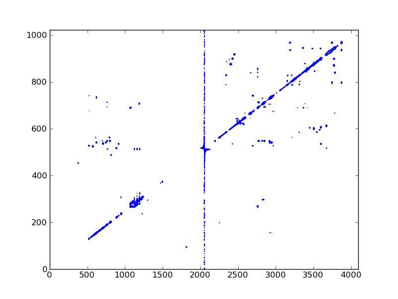

#! /usr/bin/env python

import numpy as np
import matplotlib.pyplot as plt
import nmrglue as ng

dic, data = ng.bruker.read_pdata('13/pdata/1')
cl = data.std() * 0.1 * 1.2 ** np.arange(10)
fig = plt.figure()
ax = fig.add_subplot(111)
ax.contour(data, cl, colors='blue')
fig.savefig('noesy_2d.png')