Pixar USD Python API
In this guide, we embark on a journey to explore the world of 3D geometry manipulation using the power of Python.
Our focus is on mastering the creation and editing points and faces in 3D space, with a special emphasis on utilizing the Pixar Universal Scene Description (USD) file format as our primary medium for storing and handling geometric data.
Our ultimate ambition is to pioneer "Procedural Modeling Language" (PROMO) - a concept inspired by Houdini's VEX, yet envisioned to be more high-level and robust. PROMO aims to be a versatile tool, enabling users to effortlessly create complex procedural structures, such as entire cities, with ease and precision. Imagine designing sprawling urban landscapes or intricate architectural marvels, all through the sophistication of a text-based language:
include PROMO

parameters = {'name': "Barcelona", 'size': [2, 3], 'style': "post-apocalypses"}
city = PROMO.createCity(parameters)
PROMO.saveToUSD(city)
But PROMO's vision extends beyond mere geometry creation. It's poised to become a pivotal middle layer in the evolving landscape of text-to-3D Large Language Models. By bridging the gap between linguistic expression and three-dimensional representation, PROMO sets the stage for a new era in digital content creation, where the boundaries of imagination are the only limits.

Any ambitious plan starts with the first steps. I'd like to learn the basics first.

In this chapter, we delve deep into the foundational aspects of 3D modeling, stripped away from the graphical interfaces of 3D applications. We learn the core principles that underpin the world of three-dimensional modeling, all from a Computer Science perspective. Our tool is Python, coupled with the Pixar USD file format for data storage and retrieval.
I encourage you to utilize the Solaris context of SideFX Houdini application to examine the data we produce.
Content:
- Prerequisites
- Definitions
- Create Geometry with Python
- Modify Geometry with Python
- Geometry Exporters
You will need Python 3 (I have Python 3.10) and USD Python API. Download and install Python.
Fortunately, the compiled USD Python API already exists and can be installed with pip install usd-core.
You will need Houdini, it has a fully functional free version called Apprentice.
You might want to use a Python IDE, that's very convenient, I am using Pycharm
If you are confused with Python and USD API installation, you can utilize Maya or Houdini Python editors, the latest versions of those applications comes with a USD Python API.
The Essence of 3D Models
At its core, a 3D model is a mathematical representation of objects from the real world, or even beyond the bounds of our imagination. In its simplest form, a 3D model consists of two fundamental components: geometry and materials. Our initial focus will be on the former - geometry, the very structure that shapes our models.

In 3D modeling, every creation, no matter how complex, begins with a file. This journey starts with learning how to create and save an empty USD file on the disk.
We will start with Pixar USD Hello World tutorial. Once you have USD Python API installed it is easy to build your first USD scene.
Let's save our first USD file. It would be an empty scene with one primitive named "Root":
from pxr import Usd, UsdGeom

stage = Usd.Stage.CreateNew('E:/hello_world.usda')
UsdGeom.Xform.Define(stage, '/Root')
stage.GetRootLayer().Save()
The hellow_world.usda content is pretty basic:
#usda 1.0

def Xform "Root" {}
Now we can add a sphere under the Root primitive:
from pxr import Usd, UsdGeom

stage = Usd.Stage.CreateNew('E:/hello_world.usda')
UsdGeom.Xform.Define(stage, '/Root')
UsdGeom.Sphere.Define(stage, '/Root/pixar_sphere')
stage.GetRootLayer().Save()
The resulting USD file would not be more sophisticated:
#usda 1.0

def Xform "Root"
{
    def Sphere "pixar_sphere" {}
}
If you bring this file to any application that can preview USD files (it can be Usdview, Maya, Houdini, or whatever), you will see a sphere in the viewport.
You can see/render the sphere in this file because "Sphere" is a built-in primitive defined in USD API. The actual sphere implementation, how you construct your points and polygons is hidden. Considering that our goal is to understand how to create basic polygon shapes, we can start with the reverse engineering of the simplest things.
I created a four-point plane in Houdini and saved it as a usd_plane.usda file:

Then I opened this file in the text editor and removed all information (attributes with values) that was not necessary for this plane to show up in the Houdini viewport. I removed the "orientation" and "subdivisionScheme" attributes required to display geometry correctly in all applications, but for our current task, it is fine, we get them back later. Here is what is left:
#usda 1.0

def Xform "Root"
{
    def Mesh "plane"
    {
        int[] faceVertexCounts = [4]
        int[] faceVertexIndices = [0, 1, 3, 2]
        point3f[] points = [(-1, 0, -1), (1, 0, -1), (-1, 0, 1), (1, 0, 1)]
    }
}
By examining this simple case, we can understand how geometry is represented in USDA format. We know that geometry is represented with points and faces connecting these points. Now we can see that points and faces in the USD file are defined with points, faceVertexCounts, and faceVertexIndices attributes.
When creating a 3D mesh, you first define the set of points in space. Then, using faceVertexCountsand and faceVertexIndices, you define how these points are connected to form the faces of the mesh
Points are the fundamental building blocks of any 3D mesh. The points attribute represents a list of points (or vertices) in 3D space. Each point is defined by its Cartesian coordinates (x, y, z).
The faceVertexCounts array holds the number of points in each face. For most standard meshes, faces are often triangles (3 vertices) or quadrilaterals (4 vertices). This attribute helps in determining how to group the vertices into faces. It tells the rendering system how to read the faceVertexIndices list.
The faceVertexIndices attribute is a list of indices that define which vertices make up each face of the mesh. The indices refer to the positions of vertices in the points list. By specifying the indices of vertices that form each face, you define the actual shape of the mesh. The way these indices are ordered is also important, as it determines the normals of the faces (which side is considered the 'outside' of the face).
Look at the plane screenshot from Houdini, it is easy to understand the data in the USD file:
- The faceVertexCounts array has one integer element 4, hence our mesh consists of one face with 4 points.
- The faceVertexIndices tells us the point order for our face: 0, 1, 3, 2.
- The points provides cartesian coordinates for each point, e.g. point with index 1 has (1, 0, -1) coordinates.
It is possible to define faces with just one attribute if we use a nested array (assume we need to store 2 faces):
int[] faceVertexIndices = [[0, 1, 3, 2], [4, 6, 5]]In such a case it is clear that every face is represented by a sub-array in the geometry array and we can easily determine which point belongs to which face. But this nested array structure is slow to read, so we have to "flatten" nested arrays into one, and store missing information in another attribute:
int[] faceVertexIndices = [0, 1, 3, 2, 4, 6, 5]
int[] faceVertexCounts = [4, 3]
Now we have the same data as in the nested array (e.g. we can understand how a nested array will looks like) but it is much faster to read and write.
Before we dive into the geometry creation magic, we need to extend our USD export function:
from pxr import Usd, UsdGeom, Sdf

def crate_geometry():
    """
    Procedurally create geometry and save it to the USDA file
    """

    # Create USD
    stage = Usd.Stage.CreateNew('E:/hello_world.usda')

    # Build mesh object
    root_xform = UsdGeom.Xform.Define(stage, '/Root')
    mesh = UsdGeom.Mesh.Define(stage, '/Root/Mesh')

    # Build mesh geometry. Here polygon creation magic should happen
    geometry_data = {'points': [],
                     'face_vertex_counts': [],
                     'face_vertex_indices': []}

    # Set mesh attributes
    mesh.GetPointsAttr().Set(geometry_data['points'])
    mesh.GetFaceVertexCountsAttr().Set(geometry_data['face_vertex_counts'])
    mesh.GetFaceVertexIndicesAttr().Set(geometry_data['face_vertex_indices'])

    # Save USD
    stage.GetRootLayer().Save()


crate_geometry()
We create a USDA file, add a mesh object to the Root of the USD stage, and define mesh parameters (Set mesh attributes section). The key part here is the geometry_data dictionary, which holds mesh information in our three key attributes. To create any geometry we would need to provide data for 3 key attributes: points, faceVertexCounts, and faceVertexIndices. In other words, we will develop an algorithm that injects proper data into those attributes.
As you can see, the attributes are empty, and if we run the script, the USD file will be created with 2 primitives Root and Mesh but you will not see any geometry in the viewport (you can bring the USD file from disk to a Stage context with Sublayer node):

We will focus on the mesh creation part next but for now, you can manually type attribute values to create your first Hello World hardcoded polygon!
def crate_geometry():
    """
    Procedurally create geometry and save it to the USDA file
    """

    # Create USD
    stage = Usd.Stage.CreateNew('E:/hello_world.usda')

    # Build mesh object
    root_xform = UsdGeom.Xform.Define(stage, '/Root')
    mesh = UsdGeom.Mesh.Define(stage, '/Root/Mesh')

    # Build mesh geometry. Here polygon creation magic should happen
    geometry_data = {'points': [(-1, 0, 1), (1, 0, 1), (1, 0, -1), (-1, 0, -1)],
                     'face_vertex_counts': [4],
                     'face_vertex_indices': [0, 1, 2, 3]}

    # Set mesh attributes
    mesh.GetPointsAttr().Set(geometry_data['points'])
    mesh.GetFaceVertexCountsAttr().Set(geometry_data['face_vertex_counts'])
    mesh.GetFaceVertexIndicesAttr().Set(geometry_data['face_vertex_indices'])

    # Save USD
    stage.GetRootLayer().Save()


crate_geometry()
I could never imagine that I will perform modeling by typing numbers in the text editor...

When creating procedural geometry, building points and faces separately is typically the most efficient and clear approach, especially for complex shapes like spheres or toruses.
We start from the most simple case, a cone. Despite it might seem that a polygonal plane would be easier to implement, the cone indeed is the most straightforward algorithm. Then we can move further and build other shapes.


We already discussed how to create a circle in VEX. Try to implement it by yourself with a Python node in the Houdini SOP context, it is an interesting exercise. The key here is to define the position of each point in Polar coordinates using angle and radius (we can define radius as 1 and eliminate it from the formula for simplicity) and then convert polar coordinates to cartesian using this formula:
- position X = cos(angle)
- position Y = sin(angle)
Once we have cartesian coordinates, we can create a point and set its position.
import hou
import math

geo = hou.pwd().geometry()

# Create a circle
points = 12
for point in range(points):

    angle = 2.0*3.14*point/points
    x = math.cos(angle)
    z = math.sin(angle)

    pt = geo.createPoint()
    pt.setPosition((x, 0, z))
Having a circle we just need to add one more pole point outside the loop:
import hou
import math

geo = hou.pwd().geometry()

# Create a circle
points = 12
for point in range(points):

    angle = 2.0*3.14*point/points
    x = math.cos(angle)
    z = math.sin(angle)

    pt = geo.createPoint()
    pt.setPosition((x, 0, z))

pt = geo.createPoint()
pt.setPosition((0, 1, 0))
I recommend doing it in the Houdini SOP Python node because you will see the results of your experiments right away, which is much more convenient for troubleshooting:
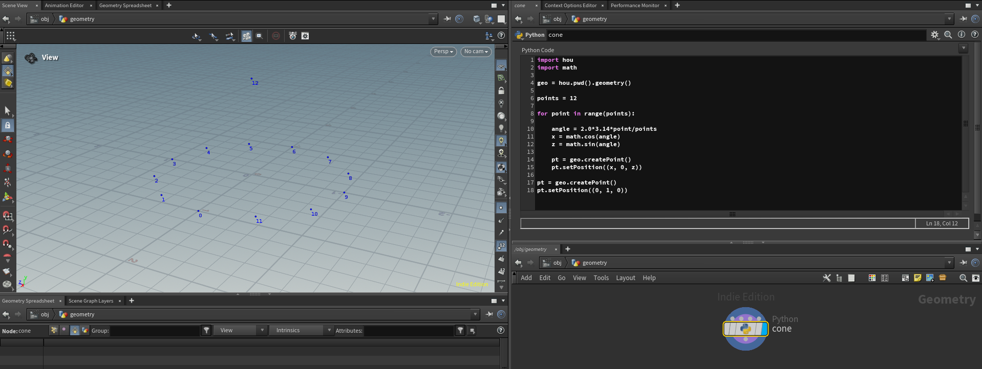
Once we get our cone points working, we can move to standalone Python, finish cone creation (we need to add polygons on top of the points) and save it to a USD file.
Let's create a cone function that will output mesh data as a dictionary of three mesh attributes:
def cone(resolution):
    """
    Create poly cone
    """

    points = []  # List of point positions
    face_vertex_counts = []  # List of vertex count per face
    face_vertex_indices = []  # List of vertex indices

    # Create geometry (points and faces) here.

    geometry_data = {'points': points,
                     'face_vertex_counts': face_vertex_counts,
                     'face_vertex_indices': face_vertex_indices}

    return geometry_data
Now in our crate_geometry() function we can call the cone() function to retrieve geometry data:
...
# Build cone geometry.
geometry_data = cone(12)
...
Let's finally implement point creation. We already did it with a SOP Python node, we just need to adjust the code a bit:
def cone(resolution):
    """
    Create poly cone
    """

    points = []  # List of point positions
    face_vertex_counts = []  # List of vertex count per face
    face_vertex_indices = []  # List of vertex indices

    # Create cone points
    for point in range(resolution):
        angle = 2.0 * 3.14 * point / resolution

        x = math.cos(angle)
        z = math.sin(angle)
        points.append((x, 0, z))

    # Add tip
    points.append((0, 2, 0))

    geometry_data = {'points': points,
                     'face_vertex_counts': face_vertex_counts,
                     'face_vertex_indices': face_vertex_indices}

    return geometry_data
Unfortunately, if we export the USD file now, we will not see any points in Houdini. We need to implement face creation. Take a look on our cone points screenshot with numbers. To build faces we need to create triangles with one tip point and two bottom points. Having 12 points as resolution, the tip point index will be 12 (we can add it last for each triangle), so we need to add such points sets to our face_vertex_indices array:
(0, 1, 12)
(1, 2, 12)
(2, 3, 12)
...
(10, 11, 12)
(11, 0, 12)
It is a simple pattern to implement:
# Crete cone faces
for point in range(resolution):
    triangle = [point, point + 1, resolution]
    face_vertex_indices.extend(triangle)
The only thing that needs to be fixed here is that on the last iteration, we will get the wrong triangle (11, 12, 12) instead of (11, 0, 12). We need to "wrap" the numbers sequence and the modulus operation will do the trick. Here you can find a modulus explanation.
Finally, we need to fill the face_vertex_counts array, and it is easy cos we will always have a triangle, so we add 3 for each iteration. Here is the final cone procedure:
def cone(resolution):
    """
    Create poly cone
    """

    points = []  # List of point positions
    face_vertex_counts = []  # List of vertex count per face
    face_vertex_indices = []  # List of vertex indices

    # Create cone points
    for point in range(resolution):
        angle = 2.0 * 3.14 * point / resolution

        x = math.cos(angle)
        z = math.sin(angle)
        points.append((x, 0, z))

    # Add tip
    points.append((0, 2, 0))

    # Crete cone faces
    for point in range(resolution):
        triangle = [point, (point + 1) % resolution, resolution]
        face_vertex_indices.extend(triangle)
        face_vertex_counts.append(3)

    geometry_data = {'points': points,
                     'face_vertex_counts': face_vertex_counts,
                     'face_vertex_indices': face_vertex_indices}

    return geometry_data
And if we put it all together in one file:
from pxr import Usd, UsdGeom, Sdf
import math


def cone(resolution):
    """
    Create poly cone
    """

    points = []  # List of point positions
    face_vertex_counts = []  # List of vertex count per face
    face_vertex_indices = []  # List of vertex indices

    # Create cone points
    for point in range(resolution):
        angle = 2.0 * 3.14 * point / resolution

        x = math.cos(angle)
        z = math.sin(angle)
        points.append((x, 0, z))

    # Add tip
    points.append((0, 2, 0))

    # Crete cone faces
    for point in range(resolution):
        triangle = [point, (point + 1) % resolution, resolution]
        face_vertex_indices.extend(triangle)
        face_vertex_counts.append(3)

    geometry_data = {'points': points,
                     'face_vertex_counts': face_vertex_counts,
                     'face_vertex_indices': face_vertex_indices}

    return geometry_data


def crate_geometry():
    """
    Procedurally create geometry and save it to the USDA file
    """

    # Create USD
    stage = Usd.Stage.CreateNew('E:/cone.usda')

    # Build mesh object
    root_xform = UsdGeom.Xform.Define(stage, '/Root')
    mesh = UsdGeom.Mesh.Define(stage, '/Root/Cone')

    # Build cone geometry.
    geometry_data = cone(12)

    # Set mesh attributes
    mesh.GetPointsAttr().Set(geometry_data['points'])
    mesh.GetFaceVertexCountsAttr().Set(geometry_data['face_vertex_counts'])
    mesh.GetFaceVertexIndicesAttr().Set(geometry_data['face_vertex_indices'])

    # Set orientation and subdivisionScheme
    mesh.CreateOrientationAttr().Set(UsdGeom.Tokens.leftHanded)
    mesh.CreateSubdivisionSchemeAttr().Set("none")

    # Save USD
    stage.GetRootLayer().Save()


crate_geometry()
Run the code and load USD file into Houdini to check if it is working:
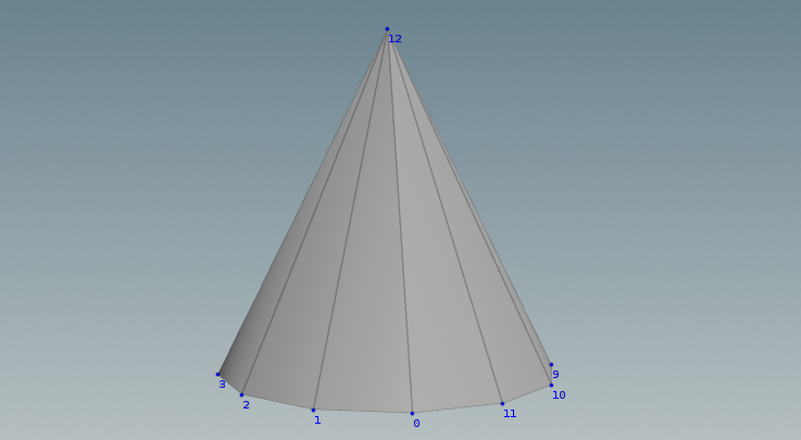
Hooray, we created the polygon shape with the help of math and programming! Now we understand better what is going under the hood in any 3D application. Now we can move to more complex shapes!

Creating a procedural sphere is also a two-stage process: generating the points and then defining the faces.
First, we focus on point creation. We will involve a bit of trigonometry and utilize polar coordinates for sphere creation. You can examine detailed description of a circle creation to get a better understanding of the math behind the code. In the case of a sphere, the difference will be in polar to cartesian coordinates conversion (we will use two angles to calculate X, Y, and Z world coordinates) and we will use 2 nested loops for point definition. Let's dive in!
Understanding Spherical Coordinates:
- Spherical coordinates are typically defined by two angles: the azimuth (θ, theta, horizontal angle) and the inclination (φ, phi, vertical angle), along with a radius (r). In our case, we disregard the radius for simplicity (assuming it is equal to 1 unit).
- The azimuth angle (θ) sweeps around the equator of the sphere, usually from 0 to 360 degrees (or 0 to 2π radians).
- The inclination angle (φ) sweeps from the top (north pole) to the bottom (south pole) of the sphere, typically from 0 to 180 degrees (or 0 to π radians).
Converting Spherical to Cartesian Coordinates:
- To place points on the sphere, you'll convert spherical coordinates to Cartesian coordinates (x, y, z) using the following formulas:
x = sin(φ) * cos(θ)y = sin(φ) * sin(θ)z = cos(φ)
Creating Points in Nested Loops:
- Use two nested loops: one for v_points (varying φ from top to bottom) and another for h_points (varying θ around the equator).
- The range of φ should be from 0 to π and the range of θ should be from 0 to 2π.
- The step size for each angle can be calculated based on the number of points (h_points and v_points).
Implement polar to cartesian coordinates conversion is simple:
def get_cartesian_position(h_angle, v_angle):
    """
    Convert polar to cartesian coordinates
    """

    position = (math.sin(v_angle) * math.cos(h_angle), math.sin(v_angle) * math.sin(h_angle), math.cos(v_angle))

    return position
Now let's build a sphere points:
def sphere(h_points, v_points):
    """
    Create polygonal sphere
    """
    # Crate sphere points
    points.append((0, 0, 1))  # Top pole

    for v_point in range(1, v_points - 1):  # Range excludes poles
        v_angle = v_point * 3.14 / (v_points - 1)

        for h_point in range(h_points):
            h_angle = 2 * h_point * 3.14 / h_points

            position = get_cartesian_position(h_angle, v_angle)
            points.append(position)

    points.append((0, 0, -1))  # Bottom pole
Until we build the entire geometry (points, and faces), we will not be able to examine intermediate results because the USD file will be incorrect and loading it into Houdini will provide no information. So for the intermediate steps, like point creation you can create a Python node in the Geometry context and write the code there, so you will access all created points in Houdini viewport. Here is the same code adapted for Python Node in the Geometry context:
import hou
import math

geo = hou.pwd().geometry()

h_points = 4
v_points = 6

def get_cartesian_position(h_angle, v_angle):

    position = (math.sin(v_angle) * math.cos(h_angle),
                math.sin(v_angle) * math.sin(h_angle),
                math.cos(v_angle))

    return position


# Top pole
top_pole = geo.createPoint()
top_pole.setPosition((0, 0, 1))


for v_point in range(1, v_points - 1):  # Range excludes poles
    v_angle = v_point * 3.14 / (v_points -1)

    for h_point in range(h_points):
        h_angle = 2 * h_point * 3.14 / h_points

        position = get_cartesian_position(h_angle, v_angle)
        point = geo.createPoint()
        point.setPosition(position)

# Bottom Pole
top_pole = geo.createPoint()
top_pole.setPosition((0, 0, -1)) 
Creating faces for a sphere involves connecting the points generated on the sphere's surface. Since we're working with a grid of points (excluding the poles), each face on the sphere (except those near the poles) will be a quadrilateral (quad). Near the poles, the faces will be triangles.
Understanding the Grid Structure:
- Visualize your sphere as a grid wrapped around it. Each quad in the grid is defined by four points: two on one latitude line and two on the adjacent latitude line.
- The grid starts from the north pole, extends down with horizontal circles (latitude lines), and ends at the south pole.
Creating Quad Faces:
- For the main part of the sphere (excluding the poles), we will create quad faces.
- We will iterate through each row (latitude) and column (longitude) to define the quads.
- Each quad is defined by four indices corresponding to its four corners: (top_left, top_right, bottom_right, bottom_left).
Handling the Poles:
- The top and bottom rows of the grid (near the poles) are special cases. Here, you'll create triangular faces instead of quads.
- Each triangle near the pole will be defined by three indices: one for the pole and two for the adjacent points on the nearest latitude line.
Implementing Face Creation:
- Start by defining the faces for the main part of the sphere.
- Then, handle the top and bottom poles separately, creating triangular faces.
def sphere(h_points, v_points):
    """
    Create polygonal sphere
    """

    points = []  # List of point positions
    face_vertex_counts = []  # List of vertex count per face
    face_vertex_indices = []  # List of vertex indices

    # Crate sphere points
    points.append((0, 0, 1))  # Top pole

    for v_point in range(1, v_points - 1):  # Range excludes poles
        v_angle = v_point * 3.14 / (v_points - 1)

        for h_point in range(h_points):
            h_angle = 2 * h_point * 3.14 / h_points

            position = get_cartesian_position(h_angle, v_angle)
            points.append(position)

    points.append((0, 0, -1))  # Bottom pole

    # Create sphere faces
    # Top pole faces
    top_pole_index = 0
    first_row_start = 1
    for h_point in range(h_points):
        next_point = (h_point + 1) % h_points
        face_vertex_indices.extend([top_pole_index, first_row_start + next_point, first_row_start + h_point])
        face_vertex_counts.append(3)

    # Main body faces (quads)
    for v_point in range(1, v_points - 2):
        row_start = 1 + (v_point - 1) * h_points
        next_row_start = row_start + h_points
        for h_point in range(h_points):
            next_point = (h_point + 1) % h_points
            face_vertex_indices.extend([row_start + h_point,
                                        row_start + next_point,
                                        next_row_start + next_point,
                                        next_row_start + h_point])
            face_vertex_counts.append(4)

    # Bottom pole faces
    bottom_pole_index = len(points) - 1
    last_row_start = 1 + (v_points - 3) * h_points
    for h_point in range(h_points):
        next_point = (h_point + 1) % h_points
        face_vertex_indices.extend([bottom_pole_index, last_row_start + h_point, last_row_start + next_point])
        face_vertex_counts.append(3)

    geometry_data = {'points': points,
                     'face_vertex_counts': face_vertex_counts,
                     'face_vertex_indices': face_vertex_indices}

    return geometry_data
Now in the crate_geometry() function change geometry_data creation to geometry_data = procedurals.sphere(8, 6), USD file name and generate a sphere.


def plane(row_points, col_points):
    """
    Create a procedural plane with a custom number of rows and columns and a size of 2.
    """

    points = []  # List of point positions
    face_vertex_counts = []  # List of vertex count per face
    face_vertex_indices = []  # List of vertex indices

    # Spacing between points
    width = 2
    height = 2
    row_spacing = height / (row_points - 1)
    col_spacing = width / (col_points - 1)

    # Generate points for the grid
    for row_point in range(row_points):
        for column_point in range(col_points):
            x = column_point * col_spacing - width / 2
            z = row_point * row_spacing - height / 2
            points.append((x, 0, z))

    # Define faces using the indices of the grid points
    for row_point in range(row_points - 1):
        for column_point in range(col_points - 1):
            # Calculate the indices of the corners of the cell
            top_left = row_point * col_points + column_point
            top_right = top_left + 1
            bottom_left = top_left + col_points
            bottom_right = bottom_left + 1

            # Define the face using the indices of the 4 corners
            face_vertex_indices.extend([top_left, top_right, bottom_right, bottom_left])
            face_vertex_counts.append(4)

    plane_data = {'points': points,
                  'face_vertex_counts': face_vertex_counts,
                  'face_vertex_indices': face_vertex_indices}

    return plane_data
Here we define a polygonal plane by generating "points", "face_vertex_counts", and "face_vertex_indices" attributes data. We do it in two stages (same as we retrieved this data from existing mesh for the exporter): create points and create faces.
The function takes a number of horizontal and vertical points as input, e.g. single quad will be created with a plane(2, 2) call.
We are building a points array with cartesian coordinates of each point. Within a nested loop iterating over rows and columns, we create a grid: first (in the "col_points" loop) one row of columns is created (points 0 and 1), then the "row_points" loop multiplies columns to get a proper number of rows (points 2 and 3). That is why we have this weird point order: 0, 1, 3, 2.
We calculate X and Z coordinates (Y will be always 0):
x = column_point * col_spacing - width / 2
z = row_point * row_spacing - height / 2
Row and column spacing are the sizes of each edge. For the horizontal (X) coordinate of each point, it will be the point number multiplied by edge length. Subtracting width / 2 from each horizontal point coordinate moves the resulting grid to the origin.
In the second part, we are getting the face_vertex_indices array that represents point order for our mesh as well as face_vertex_counts, the number of points for each face, which will be an array 4 (because each face will always have 4 points). We are using the same nested loop over rows and columns, calculate the point number for each point, and record those numbers into the face_vertex_indices array:
top_left = row_point * col_points + column_point
top_right = top_left + 1
bottom_left = top_left + col_points
bottom_right = bottom_left + 1
Each face in the grid is defined by four points: top-left, top-right, bottom-left, and bottom-right.
top_left = row * col_points + col This calculates the index of the top-left vertex of the cell. The index is determined based on the position in the grid. For example, in a 3x3 grid, the top-left point of the second cell (first row, second column) would be at index 1.
top_right = top_left + 1 The top-right vertex is simply the next one in the same row, so it's the index of the top-left vertex plus 1.
bottom_left = top_left + col_points The bottom-left vertex is directly below the top-left vertex, which means it's col_points indices away.
bottom_right = bottom_left + 1 Similarly, the bottom-right vertex is next to the bottom-left, so its index is bottom_left + 1.

Now when we can create geometry from scratch, let's see how we can do something with existing geometry and implement a simplest extrusion.
Assume we have a 4-point plane located on the XZ grid. We need to extrude it along the Y-axis at a certain distance.
points = [(-1, 0, 1), (1, 0, 1), (1, 0, -1), (-1, 0, -1)]
face_vertex_counts = [4]
face_vertex_indices = [0, 1, 2, 3]
We modify the mesh in the same way as we create it: we deal with points and then we handle faces. The extrusion algorithm would look like:
-
For each point P of the original polygon:
- Calculate new point P* = P + extrusion length
-
For each edge of the polygon:
- Consider an edge formed by points P1 and P2.
- Find the corresponding new points P1* and P2*.
- Create a new face (quad) using vertices [P1, P2, P2*, P1*].
-
Create the top face (cap):
- Use all the new points P* to create a face that is parallel to the original face.
Implementing algorithm of our hardcoded polygon in extrude_poygon function:
import copy

def extrude_polygon():
    """
    Define source poly plane with hardcoded values and perform extrusion operation on it returning new data
    """

    # Define source polygon
    points = [(-1, 0, 1), (1, 0, 1), (1, 0, -1), (-1, 0, -1)]
    face_vertex_counts = [4]
    face_vertex_indices = [0, 1, 2, 3]

    source_polygon = {'points': points,
                      'face_vertex_counts': face_vertex_counts,
                      'face_vertex_indices': face_vertex_indices}

    # Copy source polygon data to a new variable
    extruded_polygon = copy.deepcopy(source_polygon)

    # Define extrusion distance
    extrude_distance = 2

    # Loop source face points and create new points with shifted positions
    for point in source_polygon['points']:
        extruded_point = (point[0], point[1] + extrude_distance, point[2])
        extruded_polygon['points'].append(extruded_point)

    # Add face for each pair of old/new points (edges)
    source_points = len(source_polygon['points'])
    for index in range(source_points):
        lower_left = index
        lower_right = (index + 1) % source_points
        upper_right = ((index + 1) % source_points) + source_points
        upper_left = index + source_points

        quad = [upper_left, upper_right, lower_right, lower_left]

        extruded_polygon['face_vertex_indices'].extend(quad)
        extruded_polygon['face_vertex_counts'].append(4)

    # Add top face
    extruded_polygon['face_vertex_indices'].extend([7, 6, 5, 4])
    extruded_polygon['face_vertex_counts'].append(4)

    return extruded_polygon
Now we can utilize our create geometry function to save geometry modification to the USD file:
def crate_geometry():
    """
    Procedurally create geometry and save it to the USDA file
    """

    stage = Usd.Stage.CreateNew('E:/super_extrude.usda')

    # Build mesh object
    UsdGeom.Xform.Define(stage, '/Root')
    mesh = UsdGeom.Mesh.Define(stage, '/Root/ExtrudedPlane')

    geometry_data = extrude_polygon()

    mesh.GetPointsAttr().Set(geometry_data['points'])
    mesh.GetFaceVertexCountsAttr().Set(geometry_data['face_vertex_counts'])
    mesh.GetFaceVertexIndicesAttr().Set(geometry_data['face_vertex_indices'])

    # Set orientation and subdivisionScheme
    mesh.CreateOrientationAttr().Set(UsdGeom.Tokens.leftHanded)
    mesh.CreateSubdivisionSchemeAttr().Set("none")

    stage.GetRootLayer().Save()

crate_geometry()Check the geometry creation file to see how you can implement class MeshData for holding geometry information and EditMesh for manipulating geometry. In the crate_geometry() function you can run such code to extrude every third polygon of a torus.
mesh_data = geo.torus(12, 36, 2, 0.5)
edit_mesh = geo.EditMesh(mesh_data)

for i in reversed(range(12*36)):
    if not i % 3:
        edit_mesh.extrude_face(i, 0.3)

mesh_data = edit_mesh.modified_meshIt is useful to have a grasp of applications API to handle geometry. Next, we will create a super basic USD file exporters, that will be able to save only polygon data to a file.
In this part we will complete another exercise useful for understanding low-level geometry basics, we will export existing geometry to a USD file, but not directly. First, we will read mesh attribute values with application API and then we store those values in our three key attributes.
"""
Export geometry from Maya scene to USD file
"""

import random
from pxr import Usd, UsdGeom
import pymel.core as pm


def get_geometry_data(mesh):
    """
    Get points data for each face for USD file record
    """

    points = []  # World position coordinates (tuples) for each geometry point (point3f[] points)
    face_vertex_counts = []  # Number of vertices in each geometry face (int[] faceVertexCounts)
    face_vertex_indices = []  # List of geometry vertex indexes (int[] faceVertexIndices)

    # Get vertex data for each face
    vertex_index = 0
    for face in mesh.faces:
        vertex_indexes = []
        for vertex in face.getVertices():
            position = tuple(mesh.vtx[vertex].getPosition(space='world'))
            points.append(position)
            vertex_indexes.append(vertex_index)
            vertex_index += 1

        face_vertex_counts.append(len(vertex_indexes))
        face_vertex_indices.extend(vertex_indexes)

    return points, face_vertex_counts, face_vertex_indices


def process_geometry(stage, root_xform):
    """
    Iterate over all scene meshes and record them to the USD stage
    """

    for mesh in pm.ls(type='mesh'):

        # Create a USD Mesh primitive for the mesh object
        usd_mesh = UsdGeom.Mesh.Define(stage, root_xform.GetPath().AppendChild(mesh.getParent().name()))

        # Get geometry data
        points, face_vertex_counts, face_vertex_indices = get_geometry_data(mesh)

        # Set the collected attributes for the USD Mesh
        usd_mesh.GetPointsAttr().Set(points)
        usd_mesh.GetFaceVertexCountsAttr().Set(face_vertex_counts)
        usd_mesh.GetFaceVertexIndicesAttr().Set(face_vertex_indices)


def export_geometry():
    """
    Create USD file and record geometry data
    """

    # Create USD stage
    usd_file_path = f'D:/maya_geometry_{random.randint(1, 1000)}.usda'

    # Create USD stage and root object
    stage = Usd.Stage.CreateNew(usd_file_path)
    root_xform = UsdGeom.Xform.Define(stage, '/')

    process_geometry(stage, root_xform)

    # Save the USD stage to the file
    stage.GetRootLayer().Save()
    print(f'>> {usd_file_path}')


export_geometry()
We add a random suffix to the file name because if you try to export USD a second time with the same file path, it will throw an error, even if you delete the file. It can be fixed by cleaning the USD cache... later.
If we need to export geometry from the Houdini geometry context it would be even simpler. The snippet below is a basic solution, you can examine a more detailed USD exporter which includes normals, materials, and potentially other stuff.
"""
Export geometry from the Houdini geometry context.

Create a Python node in a Geometry context and connect your geometry to the first input.
"""

import random
from pxr import Usd, UsdGeom, Gf
import hou


def get_geometry_data(geometry):
    """
    Get mesh geometry data
    """

    points = []  # List of point positions (point3f[] points)
    face_vertex_counts = []  # List of vertex count per face (int[] faceVertexCounts)
    face_vertex_indices = []  # List of vertex indices (int[] faceVertexIndices)

    # Collect points
    for point in geometry.points():
        position = point.position()
        points.append(Gf.Vec3f(position[0], position[1], position[2]))

    # Collect face data
    for primitive in geometry.prims():
        vertices = primitive.vertices()
        face_vertex_counts.append(len(vertices))
        face_vertex_indices.extend([vertex.point().number() for vertex in vertices])

    return points, face_vertex_counts, face_vertex_indices


def export_geometry():
    """
    Create and save a USD file with geometry from the first input.
    """

    # Create a new USD stage
    usd_file_path = f'E:/houdini_export_{random.randint(1, 100)}.usda'
    stage = Usd.Stage.CreateNew(usd_file_path)

    # Access the input geometry
    node = hou.pwd()
    geometry = node.geometry()
    input_node = node.inputs()[0]
    input_node_name = input_node.name()

    points, face_vertex_counts, face_vertex_indices = get_geometry_data(geometry)

    # Create a USD Mesh primitive
    mesh = UsdGeom.Mesh.Define(stage, f'/Root/{input_node_name}')
    mesh.GetPointsAttr().Set(points)
    mesh.GetFaceVertexCountsAttr().Set(face_vertex_counts)
    mesh.GetFaceVertexIndicesAttr().Set(face_vertex_indices)

    # Save the stage
    stage.GetRootLayer().Save()


export_geometry()