scalableMLproject

Project in Advanced Scalable Machine Learning Course at KTH Ludvig Doeser & Xin Huang

• Group number: 26

Prediction service: the results of our TSLA stock price prediction is communicated to the interested readers with a user interface hosted at the Huggingface space: https://huggingface.co/spaces/LudvigDoeser/TSLA_stock_predictions

Predicting tomorrow's stock price of TSLA

In this project, we use time-series data (historical stock price and news sentiment data) for training a Long short-term memory (LSTM) Recurrent Neural Network model, which serves for predicting the closing stock price of Tesla, Inc. (TSLA) in the following business day. Our LSTM model is further deployed online with the Modal Stub service, which enables an automatic daily performance of the prediction of the TSLA stock price.

The workflow of this project can be factorised into the following pipelines:

• feature pipeline, which executes serverless feature engineering steps on Modal and then stores the data using Hopsworks online feature store,
  • get_historical_news_data.py and get_historical_stock_data.py grabs and pre-processes the historical data, and then saves it as .csv-files.
  • feature_preprocessing.py contains all methods of pre-processing. This script is called by all other pipelines, which prevents DRY.
  • create_and_backfill_feature_groups.py creates feature groups at Hopsworks (one for the news data and one for the stock data) and fills them with the historical data.
  • create_feature_view.py creates a feature view from the previous mentioned feature groups.
  • feature_daily.py runs once per day to grab new data points to perform inference on (see more further down).
• training pipeline, which includes (1) offline experimentation, such as neural architecture search/hyperparameter tuning using keras-tuner, and (2) the online training.
  • train_model.py contains the code for grabbing the data from the feature view, training the model with the offline found architecture/hyperparameters and uploads the trained model to the model registry at Hopsworks.
• batch-inference pipeline, which extracts newly updated stock market and news sentiment information (thanks to the feature_daily), and perform a stock price prediction for the coming business day.

Finally the results of our TSLA stock price prediction is communicated to the interested readers with a user interface hosted at the Huggingface space: https://huggingface.co/spaces/LudvigDoeser/TSLA_stock_predictions

Below we describe the different pipelines in more depth.

Feature pipelines

The raw data for our stock price prediction project consists mainly of the following two parts:

• the historical TSLA stock prices, and
• the News Sentiment data about Tesla, Inc.,

tracing from 2015-07-16 to 2023-01-10.

The historical stock price data are obtained with the yfinance package, which utilizes the Yahoo! Finance API to access the real-time market data containing the opening price, highest/lowest value, closing price, and the volume of a variety of stocks in the financial markets. The closing price data of TSLA stock and stored together with the corresponding datetime into one feature group at Hopsworks.

We have implemented tests by including more types of feature values in the training data, e.g., combining the closing price data with opening price, highest/lowest price, and volume data together, but found that employing only the closing price in the feature view could give a smallest root-mean-squre error (RMSE) for the trained LSTM model. Therefore we select only the closing price in our feature group based on this offline experimentation (see more in next section).

The News sentiment dataset is acquired from the Sentiment Data Financial API supported by EOD Historical Data, Unicorn Data Services. This dataset provides us with financial news sentiment analysis results on TSLA, which contains the date, title, specific content and link to each relevant report, together with a sentiment score for each piece of news. The news sentiment score is obtained by detection of positive and negative mentions inside one report, and normalizing them to a polarity value with scale [-1,1]. For example, a polarity value equals -1 indicates a completely negagive report, whereas +0.1 suggests a slight preference with positive attitude. The Sentiment Data Financial API updates sentiment scores direclty.

Specifically, we take the 7-day exponential moving avarage of the news sentiment scores of TSLA as one feature to be used. The exponential moving average is given by the formula

$$ y_t = {x_t+(1-\alpha)x_{t-1}+(1-\alpha)^2 x_{t-2}+\cdots+ (1-\alpha)^n x_{t-n} \over 1+(1-\alpha)+(1-\alpha)^2+\cdots+(1-\alpha)^n} $$

where $x_t$ denotes the daily observed sentiment score values, $y_t$ denotes the desired exponential moving average, $n=7$ in our case correpsonds to a 7-day time-window for exponential smoothing, and $\alpha = 2/(n+1) = 0.25 \in (0,1)$ is the smoothing factor. We may simply understand that the exponential moving average is applied to give a greater weight and significance on the most recent sentiment score data. We have also tested using $n=20$ days as the smoothing time-window, and observed similar results with using $n=7$, which validates our current choice with 7-day exponential smooothing.

After extracting the relevant information from the two raw datasets, we upload the corresponding two feature groups containing historical stock data and (smoothed) news sentiment score data respectively, to the Hopsworks feature store. Then these two feature groups are merged with the column date as the primary key to provide us with the online-embedded feature view using:

fg_query = tesla_fg.select_except(["open","low","high","volume"]).join(news_sentiment_fg.select_except(['polarity']))

In order to match the two feature groups, note that the feature view contain all dates (both business and non-business days). The feature view is further equipped with the transformation function min_max_scaler available in Hopsworks. As we only want to use business days for training, we then have a function fix_data_from_feature_view() that takes care of this.

The feature view now contains the recent TSLA stock closing price and the exponential moving average of news sentiment scores.

Training Pipeline

Our training dataset contains of sets containing the previous closing prices of the past 7 business days and the 7-day exponential moving average of the news sentiment score values. The training of our model utilizes all the accessible data to January 4th of 2023. The model we wanted to use was a LSTM Recurrent Neural Network model with adam optimization, as is given as the following create_model function:

def create_model(LSTM_filters=64,
                 dropout=0.1,
                 recurrent_dropout=0.1,
                 dense_dropout=0.5,
                 activation='relu',
                 depth=1,
                 input_channels=1):

    model = Sequential()
    
    if depth>1:
        for i in range(1,depth):
            # Recurrent layer
            model.add(LSTM(LSTM_filters, return_sequences=True, dropout=dropout, recurrent_dropout=recurrent_dropout,input_shape=(timelag, input_channels)))

    # Recurrent layer
    model.add(LSTM(LSTM_filters, return_sequences=False, dropout=dropout, recurrent_dropout=recurrent_dropout, input_shape=(timelag, input_channels)))
    
    # Fully connected layer
    if activation=='relu':
        model.add(Dense(LSTM_filters, activation='relu'))
    elif activation=='leaky_relu':
        model.add(Dense(LSTM_filters))
        model.add(keras.layers.LeakyReLU(alpha=0.1))

    # Dropout for regularization
    model.add(Dropout(dense_dropout))

    # Output layer
    model.add(Dense(1, activation='linear'))

    # Compile the model
    model.compile(optimizer='adam', loss='mse')
    
    return model

model = create_model(activation='relu',input_channels=2,depth=2)

(1). Offline experimentation and Training of the LSTM model (see more in the tuning_network-directory)

For the training of our LSTM Recurrent Neural Network model, we apply a Bayesian optimization-based search for the setting of hyperparameters, with the help of the KerasTuner tool. Specifically we use 0.1 for the validation split ratio and 256 for the batch size. The hyperparameter values of the three best trials which returns the smallest RMSE values are summarized in the following table.

RMSE	No. filters	dropout rate	recurrent_dropout	dense_dropout	depth	activation function
0.00125	128	0.01	0.1	0.01	1	leaky-relu
0.00134	128	0.01	0.3	0.01	1	leaky-relu
0.00138	128	0.01	0.01	0.01	1	leaky-relu

One example of our training and validation error for the best hyperparameter setting in the above table are plotted as follows.

The predicted TSLA stock prices (in blue) using our trained model, with the true historical stock prices (in red) are shown in the following figure.

(2). Serverless training with Modal

We end up using a model that was trained for 179 epochs, with validation split ratio of 0.1 (with different random seed value from the hyperparameter tuning) and applying early stopping.

By connecting with Modal and using the data from our online feature view, the training can be performed online through the Modal Stub service on a regular basis. Please see also the script named 'train_model.py'.

Our model obtained from the above training steps is uploaded to the Hopsworks Model Registry.

Batch Inference Pipeline

Since the News Sentiment dataset is updated regularly (as the news are published) and the Nasdaq stock market closes at 21:00 (Greenwich time), our Feature daily pipeline is scheduled to be launched at 21:05 of Greenwich time every day. We acquire the newly updated closing price data and News sentiment data, through the Yahoo! finance API and the Sentiment Data Financial API respectively. The feature_daily.py also writes the obatined new production data into our feature groups, and avoids concerns about DRY code by the use of the same pre-processing steps (as for the historical data) and transformations (through the feature view). The real-time data are combined with the most recent 7-day historial data which are retrived from the feature view. These new features can thus be inserted into our online feature view, aggregating the newly updated information for today and computing the new exponential moving average.

Moreover, we get the trained model from Hopsworks Model Registry and grab the data from the Hopsworks feature view. Then we are able to implement a prediction based on the newly obtained feature values, and our new prediction for the next business day is communicated through a UI based on our huggingface space. Specifically, we provide a table containing the predictions and true closing stock prices in the past 5 days, comparing the predicted increase/decrease in the price v.s. the true changes in the value.

The information of this Table is also visualized with a corresponding figure, which also plots the predicted price of the next business day.

This Batch Inference/Prediction Pipeline is also deployed on Modal. By specifying the schedule at 21:45 of each day for the stub.function with the modal.Cron function, our TSLA stock price prediction is performed automatically on every evening for the upcoming businessday, based on the newly obtained news sentiment scores and the closing stock price of today.

Scheduled programs at modal:

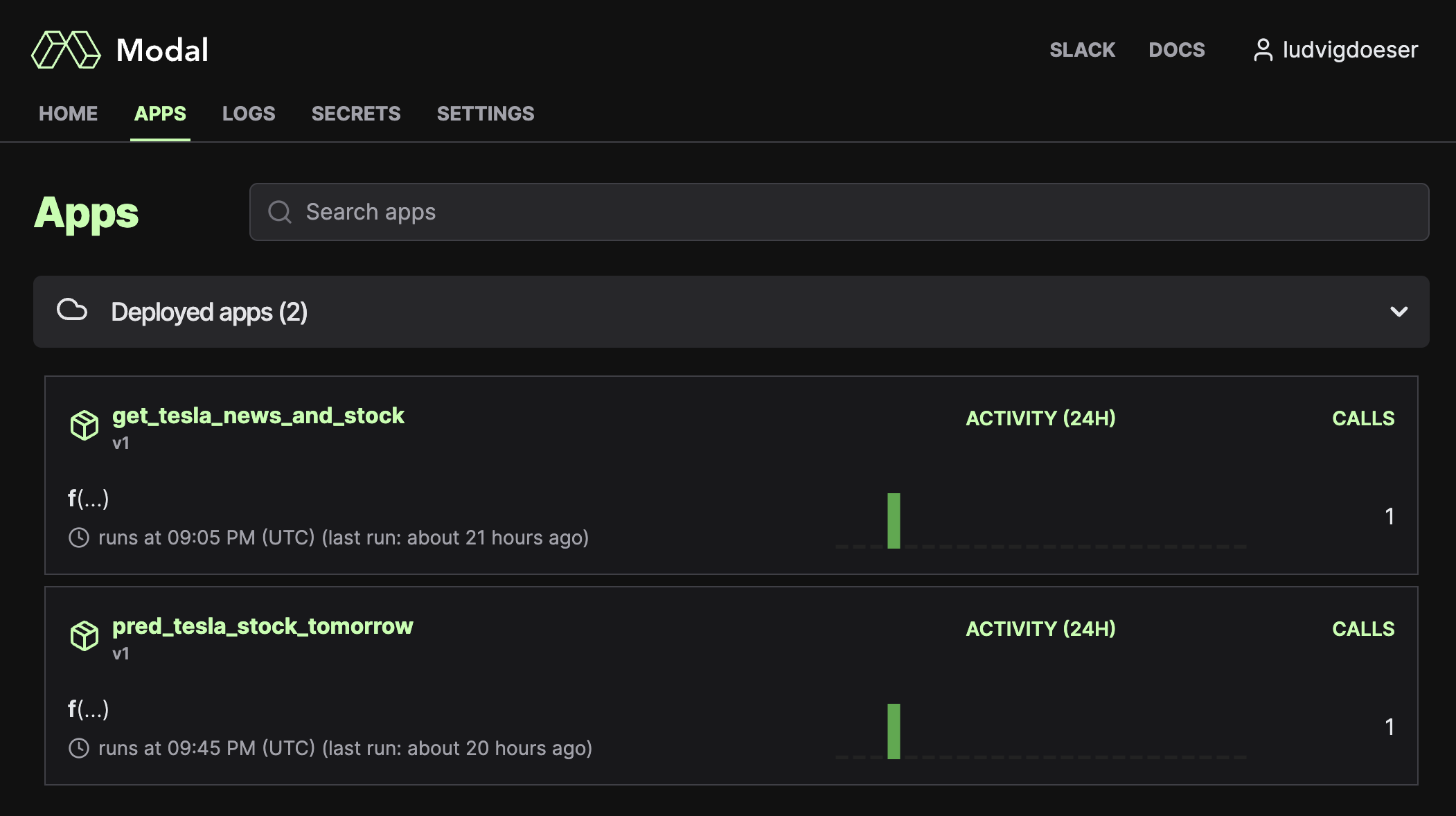
We deployed the scripts using:

modal deploy --name get_tesla_news_and_stock feature_daily.py
modal deploy --name pred_tsla_stock_tomorrow batch_inference.py

As we can see, they make 1 call each per day:

Inspiration

• https://www.projectpro.io/article/stock-price-prediction-using-machine-learning-project/571
• https://stocksnips.net/learn/news-based-stock-sentiment/
• https://towardsdatascience.com/sentiment-analysis-on-news-headlines-classic-supervised-learning-vs-deep-learning-approach-831ac698e276
• https://github.com/logicalclocks/hopsworks-tutorials/tree/master/advanced_tutorials
  • In particular, this one: https://github.com/logicalclocks/hopsworks-tutorials/tree/master/advanced_tutorials/bitcoin
• https://github.com/featurestoreorg/serverless-ml-course

Requirements for running the code

Download the repo, create a new conda environment and then run:

pip install -r requirements.txt

For the interested reader, one can create a pip3 compatible requirements.txt file using:

pip3 freeze > requirements.txt  # Python3