Functional diversity of microbial eukaryotes in a meromictic lake: coupling between metatranscriptomic and a trait-based approach
This is a workflow to reproduce analysis conduced in Monjot et al., 2023
First, clone github repository: git clone https://github.com/meb-team/MICROSTORE_MetaT-MetaB_Monjot_2023.git
Second, define current directory: cd MICROSTORE_MetaT-MetaB_Monjot_2023
                                    *******************************
                                        Directory organization
                                    *******************************
Microstore_Analysis_Monjot_et_al._2023
|-> rawdata (sub-directory for reads, traits table, metadata)
    |-> metadata_metaB (metadata of metabarcoding data)
    |-> metadata_metaT (metadata of metatranscriptomic data)
    |-> BTTwellannoted.csv (Marine traits table by Ramond et al., 2019)
    |-> Table_Supp_1.tsv (own traits table (Monjot et al., 2023))
    |-> ko_to_hierarchy.txt (KO id definition table from https://www.genome.jp/kegg-bin/show_brite?ko00001.keg)
|-> script (sub-directory for minor scripts)
    |-> 0_download_metaB_data.sh (script for downloading metabarcoding raw reads)
    |-> 1_Pre-process.sh (pre-processing script)
    |-> 2_Orient_reads_parallel.sh (script to launch parallelization of reads reorientation script)
    |-> 2_Orient_reads.py (reads reorientation script)
    |-> 3_Install_dependencies.R (dependencies installation script)
    |-> 4_Dada2.R (DADA2 pipeline script)
    |-> 5_Analyse_Composition_ASV_DADA2.R (script to analyze taxonomic diversity)
    |-> 6_Preview_Tax_ref.R (script to extract taxonomic ref in order to launch trait-based analysis)
    |-> 7_Calcul_Rarecurve.R (script to process rarefaction curve and diversity index)
    |-> 8A_Kmean_Clusterization.R (script to clusterize taxonomic references using custom traits table)
    |-> 8B_Analyse_Function_Table.R (script to start trait-based analysis using previously defined cluster names)
    |-> 9_Duplicat_Metatrans_analize.R (script to start comparison between duplicates of conditions)
    |-> 10_KO_Metatrans_DESeq2.R (DESeq2 pipeline script)
    |-> environment_REnv_Monjot_2023A.yml (conda environment)
    |-> REnv_Monjot_2023A_packages (local repository to R packages installation)
|-> Preprocess_setup.sh (script to launch conda environment setup)
|-> Downloading_metaB_rawdata.sh (script to launch  metabarcoding raw reads download)
|-> Downloading_metaT_rawdata.sh (script to launch  metatranscriptomic catalog genes download)
|-> DADA2_1_preprocess.sh (script to launch the preprocessing stage)
|-> DADA2_2_reorient_py.sh (script to launch raw reads reorientation)
|-> R_3_setup.sh (script to launch R dependencies installation scripts)
|-> R_4_DADA2_process.sh (script to launch DADA2 pipeline)
|-> R_5_Taxonomic_analysis.sh (script to launch Taxonomic diversity analysis)
|-> R_6A_Kmean_Clusterization.sh (script to launch kmean clusterization)
|-> R_6B_Functional_analysis.sh (script to launch Trait-based analysis)
|-> R_7_Metatranscriptomic_analysis.sh (script to launch DESeq2 pipeline and metatranscriptomic analysis)
|-> Retrieve_Figures.sh (script to retrieve published figures from result directory)
|-> V4-DADA2.ini (initialization file for metabarcoding analysis)
|-> MetaT.ini (initialization file for metatranscriptomic analysis)
Raw reads is downloaded from ENA archive under PRJEB61527 accession number:
bash Downloading_metaB_rawdata.sh
- script: Downloading_metaB_rawdata.sh
The compressed paired end reads (R1.fastq.gz and R2.fastq.gz) are automatically placed in a reads/ sub-directory in rawdata/ directory.
*******************************
    Sampling nomenclature
*******************************
Sampling name example : DJAG_04_2
with :
1. Molecule type        ADN    D
2. Daylight        JOUR:J    NUIT:N
3. Oxygen        OXIQUE:O    ANOXIQUE:A
4. Fraction        G:10-50    P:INF10
5. Date        04    06    09    11
6. Replicate        RIEN OU 1    2

*******************************
    Run name nomenclature
*******************************
Run name example : 191029_MELISSE_D78BK
with :
1. Date : 191029
2. Sequencer : MELISSE
3. Flowcell id : D78BK
Other sequencer names : MELISSE MIMOSA PLATINE

*******************************
    Paired files nomenclature
*******************************
Name file examples :
CIN_CBOSTA_1_1_D78BK.12BA207_clean.fastq.gz
CIN_CBOSTA_1_2_D78BK.12BA207_clean.fastq.gz
with :
1. Project code : CIN
2. Material name : CB
3. Sequencing type : S = Solexa
4. Bank type : TA : TA - Targeted DNAseq
5. Lane number : 1
6. Read number : 1
7. Flowcell id : D78BK
8. Index : 12BA207

*******************************
    Sequence header nomenclature
*******************************
Sequence name example :
@M1:A6U0C:1:1101:17317:1262/2
@H3:C29DNACXX:2:1101:1349:2239/1
with :
1. Sequencer id : @M1 ; M = Miseq; H = Hiseq
2. Flowcell id : A6U0C
3. Lane number : 1
4. Tile number : 1101
5. x coordinate on the tile : 17317
6. y coordinate on the tile : 1262
A table containing the name ("DM", "DN", etc.), the condition (DNOG, DJAP, etc.), the date (04, 06, 09 or 11), the region (V4) and replicate ID (1 or 2) corresponding to each amplicon is needed.
- We provides the following table: metadata_metaB which is located in the rawdata/ directory.
Install miniconda following the standard procedure (https://docs.conda.io/projects/miniconda/en/latest/miniconda-install.html)
Then, install conda environment with the following script:
bash Preprocess_setup.sh
- script: Preprocess_setup.sh
- This takes 1 min on [Dual CPU] Intel(R) Xeon(R) CPU E5-2670 with 512 Go of RAM
This installs the following tools:
* KronaTools v2.8
* cutadapt v4.1
* r-base v4.2.2
* imagemagick v7.1.0_52
* python v3.9.15
* perl v5.32.1
* cmake v3.22.1
* parallel v20230722
* numerous libraries (details in script/environment_REnv_Monjot_2023A.yml)
To start DADA2 analysis, the reads must be pooled according to their replicates ID.
Run pre-processing script :
bash DADA2_1_preprocess.sh
- script: DADA2_1_preprocess.sh
- This takes just a few seconds on [Dual CPU] Intel(R) Xeon(R) CPU E5-2670 with 512 Go of RAM
At the end of this stage, some result files are generated : V4 and V4-unified ; respectively reads V4 not pooled and the reads V4 pooled. These files are created in reads/ sub-directory located in dataDADA2/ directory (also created at this stage).
Reads must be re-orient for ASV processing. In fact, Illumina adaptators are randomly linked to the DNA fragments during sequencing process and the reads R1 and R2 are represented by approximately 50% of forward reads and 50% of reverse reads.
To complete this, run following script :
bash DADA2_2_reorient_py.sh V4-unified 16 "GTG[CT]CAGC[AC]GCCGCGGTA" "TTGG[CT][AG]AATGCTTTCGC"
- script: DADA2_2_reorient.sh
- argument 1: input file for reorientation (V4 or V4-unified)
- argument 2: number of threads to process data
- argument 3: forward primer
- argument 4: reverse primer
- This takes 1 min on [Dual CPU] Intel(R) Xeon(R) CPU E5-2670 with 512 Go of RAM
Install R dependencies with the following script:
bash R_3_setup.sh
- script: R_3_setup.sh
- This takes 77 min on [Dual CPU] Intel(R) Xeon(R) CPU E5-2670 with 512 Go of RAM
This operation installs the following R packages:
* GUniFrac              * reshape2                  * vegan
* ggplot2               * SARTools                  * gtools
* tidyr                 * ComplexHeatmap            * SciViews
* dplyr                 * DESeq2                    * paletteer
* cowplot               * dada2                     * cluster
* ggrepel               * elementalist              * stringr
* ggsci                 * ggh4x                     * NbClust
* scales                * R.utils                   * BiocManager
* varhandle             * scatterplot3d             * tibble
* treemap               * car                       * svglite
* VennDiagram           * rgl                       * treemapify
* FactoMineR            * data.table                * hrbrthemes
* RColorBrewer          * devtools                  * psych
* factoextra            * ggExtra                   * ggpubr
* reshape2              * gplots
Initialization file .ini is created from the V4-DADA2.ini:
For example:
## Raw data directory [1]
INPUT    V4-unified-correct-paired

## Database [2]
DATABASE    pr2_version_4.14.0_SSU_dada2.fasta.gz

## Result directory [3]
RESULT    V4-unified-correct-paired-out

## Minimum read length [4]
MINLEN    200

## Maximum read length [5]
MAXLEN    500

## Maximum N nucleotide in reads [6]
MAXN    0

## Minimum of the overlap region between forward and reverse reads [7]
MINOVERLAP    50

## Mismatch value accepted on the overlap region between forward and reverse reads [8]
MAXMISMATCH    0

## Number of threads to process data [9]
NTHREADS    16

## Primer Forward [10]
FWD    GTGYCAGCMGCCGCGGTA

## Primer Reverse [11]
REV    TTGGYRAATGCTTTCGC

## Region [12]
REGION    V4

## Filter (if yes enter filter mode : "Bokulich", "Singleton", "Doubleton" or "OnlyOne" ; if no enter "no") [13]
FILTER    Singleton

## Rarefy global data (yes or no) [14]
RAREFY    yes

## Rarecurve Calcul (yes or no) ? It make a while [15]
RARECURVE    yes

## Process Composition script (yes or no) [16]
COMPOSITION    yes

## Output for the Composition script [17]
OUTCOMP    V4-unified-correct-paired-out-compo
Run DADA2 workflow:
bash R_4_DADA2_process.sh V4-DADA2.ini
- script: R_4_DADA2_process.sh
- argument 1: V4-DADA2.ini
- This takes 84 min on [Dual CPU] Intel(R) Xeon(R) CPU E5-2670 with 512 Go of RAM
Run Taxonomic analysis script:
bash R_5_Taxonomic_analysis.sh V4-DADA2.ini
- script: R_5_Taxonomic_analysis.sh
- argument 1: V4-DADA2.ini
- This takes 35 min on [Dual CPU] Intel(R) Xeon(R) CPU E5-2670 with 512 Go of RAM
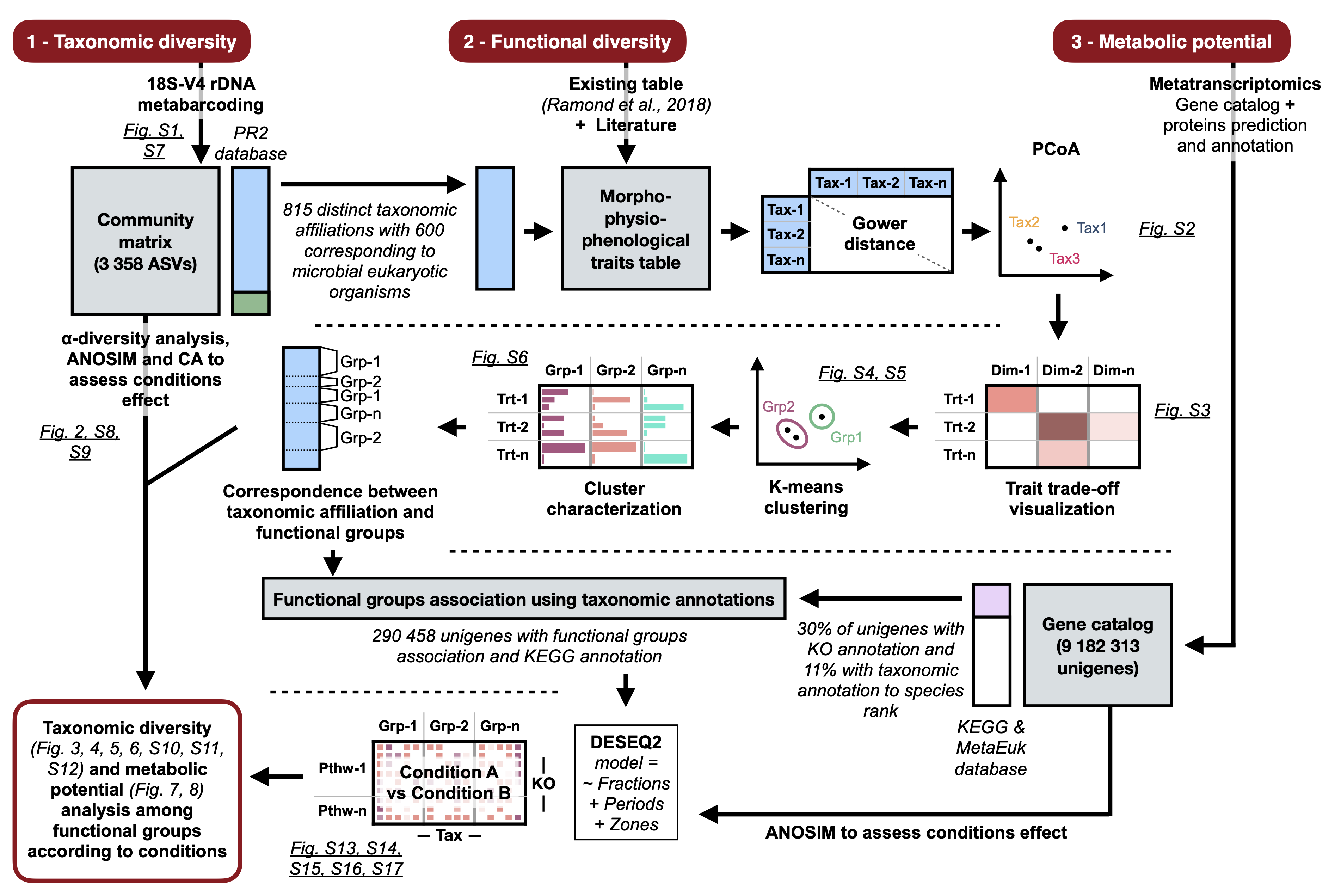
Previous steps annotate taxonomic references using marine traits table provided by Ramond et al., 2019. The resulting table is generated in result/ sub-directory which is located in dataDADA2/ directory.
Prepare your traits table using the previously generated table and place it on rawdata/ directory in .tsv format or use our trait table already present in rawdata/ directory: Table_Supp_1.tsv.
Run kmean clusterization to define clusters:
bash R_6A_Kmean_Clusterization.sh Table_Supp_1.tsv V4-unified-correct-paired-out-compo V4
- script: R_6A_Kmean_Clusterization.sh
- argument 1: name of the trait table in tsv format
- argument 2: name of the taxonomic analysis results directory
- argument 3: Region (V4 or V9)
- This takes just a few seconds on [Dual CPU] Intel(R) Xeon(R) CPU E5-2670 with 512 Go of RAM
This operation produces a cluster_name.tsv table providing the number of clusters as well as a Def_group_by_factor.svg figure in rawdata/ directory. You have to complete the .tsv file with names of clusters using the Def_group_by_factor.svg figure.
In Monjot et al. 2023, authors characterized clusters using modalities of each morpho-physio-phenological trait. The functional groups have been named consequently: 1&5) Parasites (PARA): characterized by their feeding strategy, symbiosis type (the majority has been described as having a parasitic lifestyle) and organic covers or naked; 2) Saprotrophs (SAP): characterized by saprotrophic feeding strategy, attached lifestyle and mainly absence of biotic interaction reported in the literature; 3) Heavy-cover- and Swimmer-photoautotrophs (HCOV and SWAT): characterized by plastids presence and osmotrophic ingestion mode with either mineral cover (e.g. siliceous) and non-swimming abilities or organic cover and swimming abilities; 4&7) Strict-heterotrophs (HET): characterized by phagotrophic feeding strategy and the absence of plastids; 6) Mixoplankton (MIXO): considered as photo-osmo-phago-mixotrophs according to Mitra et al. (2023) and characterized by the presence of chloroplast, motility and their feeding strategy (Phagotrophic in majority); 8) Floater- and colonial-photoautotrophs (FLAT): characterized by non-swimming abilities, plastids presence and osmotrophic ingestion mode; 9) Endophyte (END): characterized by their attached life-style, feeding strategy, biotic interaction with plants and mostly organic covers.
For example:
nbGroup	name
Cluster 1	PARA
Cluster 2	SAP
Cluster 3	HCOV and SWAT
Cluster 4	HET
Cluster 5	PARA
Cluster 6	MIXO
Cluster 7	HET
Cluster 8	FLAT
Cluster 9	END
Then, run functional analysis script:
bash R_6B_Functional_analysis.sh Table_Supp_1.tsv V4-unified-correct-paired-out-compo V4
- script: R_6B_Functional_analysis.sh
- argument 1: name of the trait table in tsv format
- argument 2: name of the taxonomic analysis results directory
- argument 3: Region (V4 or V9)
- This takes 3 min on [Dual CPU] Intel(R) Xeon(R) CPU E5-2670 with 512 Go of RAM
Unigenes catalog as well as taxonomic and functional annotations were downloaded from ZENODO archive (available under https://doi.org/10.5281/zenodo.8376850 DOI link): bash Downloading_metaT_rawdata.sh
- This script downloads unigenes table (with functional annotations) and taxonomy table: respectively main_table.mapping.unique.read_per_kb.noHuman.noConta.noMetazoa.annot.tsv and table_taxonomy.perUnigene.allUnigenes.tsv.
The generation of these files (i.e. taxonomy and functional annotations) are described below.
Metadata file as well as KO id definition table must be placed in rawdata/ directory.
- We provide the following metadata table: metadata_metaT as well as KO id definition table generated from https://www.genome.jp/kegg-bin/show_brite?ko00001.keg .
Initialization file .ini is then create from the MetaT.ini:
For example:
## Enter unigene table (.tsv) (located in rawdata directory) [1]
INPUT    main_table.mapping.unique.read_per_kb.noHuman.noConta.noMetazoa.annot.tsv

## Result path (the same of the composition script output) [2]
OUTPUT    V4-unified-correct-paired-out-compo

## Unigene Taxonomy path (located in rawdata directory) [3]
TAX    table_taxonomy.perUnigene.allUnigenes.tsv

## Database path used in the trait study (located in database directory) [4]
DATABASE    pr2_version_4.14.0_SSU_dada2.fasta.gz
Then, run metatranscriptomic analysis script:
bash R_7_Metatranscriptomic_analysis.sh MetaT.ini
- script: R_7_Metatranscriptomic_analysis.sh
- argument 1: MetaT.ini
- This takes 294 min (≈5 hours) on [Dual CPU] Intel(R) Xeon(R) CPU E5-2670 with 512 Go of RAM
The raw data are available in the public databases under the umbrella of the BioProject PRJEB61515. There are 32 samples, each of them assembled one-by-one with oases and were clustered all together with CD-HIT-EST with the thresholds identity >95% over >90% of the length of the smallest sequence. Moreover, transcripts longer than 50kb were discarded, this resulted in 10.359.104 representative assembled transcripts, called herafter Unigenes. The protocol is described in grater details in the work from Carradec et al. 2018.
We then removed human contamination from the Unigenes. Unigenes were aligned to the Human genome assembly GRCh38.p13 with minimap2 v2.14-r894-dirty and the default parameters. All Unigenes with a hit against the genome weere considered as contaminant as thus discarded for future analysis. Here is an example of code to obtain the list of contaminants:
minimap2 -t 12 GRCh38.p13.genome.fa.gz Unigenes.fa | cut -f 1 | sort | \
    uniq >list_unigene_human_contaminant
A total of 32.218 Unigenes were discarded.
We used TransDecoder v5.5.0 to predict coding sequences present on the Unigenes. The minimal protein length was set to 70 amino-acids as we observed Unigenes without protein with the default parameters:
# Extract long Open-Reading Frames
TransDecoder.LongOrfs -m 70 --output_dir out_transDecoder -t unigenes.fa

# Predict the likely coding regions
TransDecoder.Predict --output_dir out_transDecoder -t unigenes.fa

# Clean the deflines
sed -i "s/ \+$//" unigenes.fa.transdecoder.pep
Proteins have been check against the AntiFam database and HMMER v3.3.2 using the profiles' score cutoff. Spurious proteins were then discarded:
# Resources:
wget ftp://ftp.ebi.ac.uk/pub/databases/Pfam/AntiFam/current/Antifam.tar.gz
tar -zxf Antifam.tar.gz

# Run the comparison: only positive hits
hmmsearch --cut_ga --noali --tblout antifam_search.tsv AntiFam.hmm proteins.faWe used MetaEuk version commit 57b63975a942fbea328d8ea39f620d6886958eca. The taxonomic affiliation is based on the database provided by MetaEuk authors, available here. This web-page proposes a link to download the data as well as a complete description of the origin of data. Beware the database is a 20 GB tar.gz archive that takes up to 200 GB of disk-space once uncompressed.
MetaEukTaxoDB=MMETSP_zenodo_3247846_uniclust90_2018_08_seed_valid_taxids

# Create the 'MMSeqs' database
metaeuk createdb unigenes.fa UnigeneDB

# Search the taxonomy for each protein
metaeuk taxonomy UnigeneDB $MetaEukTaxoDB Unigene_taxoDB tmp \
    --majority 0.5 --tax-lineage 1 --lca-mode 2 --max-seqs 100 -e 0.00001 \
    -s 6 --max-accept 100

# Get a Krona-like plot
metaeuk taxonomyreport $MetaEukTaxoDB Unigene_taxoDB \
    Unigene_report.html --report-mode 1

# Get a tsv
metaeuk createtsv UnigeneDB Unigene_taxoDB \
    Unigene_taxonomy_result.tsv
Then we associated the taxonomy of the protein to its corresponding Unigene. In the case where a single protein is present on a Unigene, we simply transfered the taxonomic annotation. Otherwise we applied this strategy:
- one or many unclassified proteins and a single affiliated protein, we transfer the affiliation as is
- at least two affiliated protein proteins: Lowest Common Ancestor strategy
This step is performed with the script metatrascriptome_scripts/map_taxo_to_unigene.py:
python3 metatrascriptome_scripts/map_taxo_to_unigene.py \
    -i Unigene_taxonomy_result.tsv \
    -b unigenes.fa.transdecoder.bed \
    -o Unigene_taxonomy_result.per_Unigene.tsv
It is important to note that Unigenes without predicted proteins are not present in this file.
From the taxonomic information, Unigenes affiliated to Bacteria, Archaea
or Viruses were removed, representing approximatly 250.000 Unigenes.
As our focus is on single-cell eukaryotes, about 150.000 Unigenes affiliated to
Metazoans have been discarded.
Proteins have been annotated with the KEGG's KO through the tool koFamScan v1.3.0 using the KO HMM profiles release "2022-01-03", available here.
# Get data
wget https://www.genome.jp/ftp/db/kofam/archives/2022-01-03/ko_list.gz
gunzip ko_list.gz
wget https://www.genome.jp/ftp/db/kofam/archives/2022-02-01/profiles.tar.gz
tar -zxf profiles.tar.gz

# Run
exec_annotation -o results.koFamScan.tsv --format detail-tsv --ko-list ko_list\
    --profile profiles proteins.fa
Then, we sent the results to the Python3 script
metatrascriptome_scripts/parse_ko_hits.py:
python3 parse_ko_hits.py --input results.koFamScan.tsv \
    --output results.koFamScan.parsed.tsv
This script parses the results in this order of preference:
- Keep hit if tagged as significant by KoFamScan, the ones with a
*in the first field. This type of result is tagged with "significant" in the result - If the current protein has no significant hit, keep the best hit if its e-value is ≤ 1.e-5.
We search all proteins agains the PfamA database, release 35.0, with HMMER v3.1b2. We used the profile's scores to determine significant hits:
hmmsearch --cut_ga --noali --tblout results.pfam.txt Pfam-A.hmm \
    proteins.fa
Then, we sent the results to the Python3 script
metatrascriptome_scripts/parse_pfam_hits.py:
python3 parse_pfam_hits.py --input results.pfam.txt \
--ouput results.pfam.parsed.tsvTo retrieve article figures, run following script:
bash Retrieve_Figures.sh V4-unified-correct-paired-out-compo
- script: Retrieve_Figures.sh
- argument 1: V4-unified-correct-paired-out-compo
- This takes just a few seconds on [Dual CPU] Intel(R) Xeon(R) CPU E5-2670 with 512 Go of RAM
The resulting figures can be found in Monjot_etal_2023/ directory.