Building Energy Consumption

Introduction

This is a data engineering project based on the Google Cloud Platform, specifically utilizing the Pub/Sub-Dataflow-BigQuery serverless stream processing. The raw data was sourced from Schneider Electric Exchange, under "Buildings energy consumption measurements" There are two problems that this project aims to solve:

1. Batch load each building's energy consumption data for data analysts or data scientists to perform analysis.
2. Calculate the average energy consumption of each building in real time and provide the data in real time for monitoring.

Table of Contents

1. Architecture
2. Data Simulation
3. Data Pipeline
4. Results
5. How To Run on GCP
6. Further Improvements
7. Licensing

Architecture

• Ingestion Layer (Compute Engine, Cloud Pub/Sub):

  • In a realistic scenario, the sensor to Pub/Sub architecture would look something like this:

    
    Source: "Using Cloud IoT Core gateways with a Raspberry Pi"

  • Since the original data is a historical data of the energy consumption, a compute engine instance was used to simulate the ingested data published to Cloud Pub/Sub architecture.

• Batch Layer (Cloud Dataflow): With the Apache Beam's PubsubIO, the messages published from the ingestion layer were read, translated into BigQuery rows, and were loaded to BigQuery.

• Streaming Layer (Cloud Dataflow): On top of ingesting the data using PusubIO with the batch layer, the real time analysis of running average of the main meter readings of each building was conducted. The results were both stored in BigQuery and also published to a separate topic on Cloud Pub/Sub in case of creating a web interface for serving the real time data publicly.

• Serving Layer (BigQuery, Cloud Pub/Sub): As mentioned in both batch layerand streaming layer, the historical data and real time data were stored in BigQuery for quick data access or analysis and the real time data was also published to Cloud Pub/Sub as a source for streaming ingestion of running average values, in case for a UI in the future.

Data Simulation

Structure of the Original Data

As seen on the original csv exported from Schneider Electric Exchange, the original schema of the csv was:

Timestamp	1_Main Meter_Active energy	1_Sub Meter Id1_Active energy	...	8_Sub Meter Id9_Active energy
2017-04-02T02:15:00-04:00	17779.0	3515.0	...	361.0

The timstamp used the UTC ISO format, and the energy readings were taken every fifteen minutes, read in Watt-hour.

Restructured Raw Data for Simulation

Since the original data was cleaned manually and all of the building data were gathered into a single table by whoever posted the data on the online library, I wanted to adjust the schema to something more realistic in a scenario where multiple sensors from multiple buildings were sending their data. I assumed that the IoT Gateway that I tried to simulate received the data on building to building basis, and performed the most minimal function possible to reach Cloud Pub/Sub (e.g. gathering multiple sensor data with common building location to be aggregated into a single row). Example schema of building 1 and building 8 are shown below:

timestamp	building_id	Gen	Sub_1	Sub_3
YYYY-MM-DD HH:MM:SS.SSSSSS	1	17779.0	3515.0	1942.0

timestamp	building_id	Gen	Sub_1	Sub_10	Sub_11	Sub_9
YYYY-MM-DD HH:MM:SS.SSSSSS	8	16039.0	4471.0	253.0	2938.0	361.0

Pub/Sub, SpeedFactor, and Event Timestamps

When running the send_meter_data.py to lauch the data publishing simulation to Pub/Sub, the user must provide the speedFactor. The speedFactor allows the user to quicken the simulation of data. For example, if the user provides the SpeedFactor of 60, one event row of the original data will be sent per minute. More accurately, after the change in the schema, 8 rows will be published per minute (although the order of arrival of the messages won't be the same every time due to latency). To match the original data time increment, the user must provide the SpeedFactor of 900, meaning one event per 15 minutes.

Along with splitting the original rows of data in send_meter_data.py as explained in Restructured Raw Data for Simulation, event timestamps were altered to match real time prior to publishing on Pub/Sub to reflect the appropriate real time behavior.

Data Pipeline

The Dataflow DAG above provides the step by step view of how the data was ingested, aggregated, and loaded, or stream inserted. Starting from the top, the data was read and ingested from Cloud Pub/Sub. Then, the pipeline was branched to the stream (on the left), and batch (on the right) processing.

Stream Processing

In the stream processing, the SlidingWindows was set, and the general meter readings of each building was aggregated according to the window created to calculate the Mean. The SlidingWindows took two requird arguments -- size and period. The size indicates how wide the window should be in seconds, and the period indicates for how long (in seconds) the aggregation must be recalculated. A sliding window of 60 seconds with period of 30 seconds would look something like this:

Source: "Beam Programming Guide"

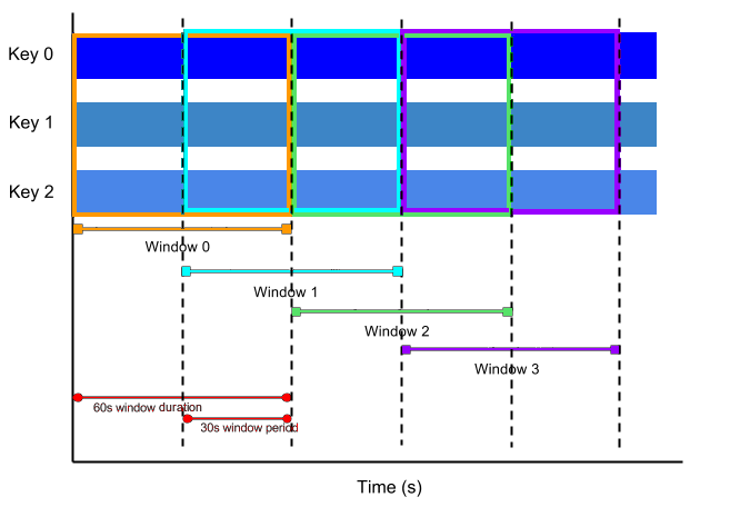
The SlidingWindows on an hourly basis with period of half an hour was specifically chosen instead of a regular FixedWindows, because the default FixedWindows waits until the end of the window to produce the aggregation results. Since the aim of the stream pipeline was to calculate the real time average of the energy readings, the SlidingWindows was chosen.

After the aggregation, the pCollection was again split into two pipelines, one to load the data to BigQuery for later analysis, and the other to publish to Pub/Sub to allow the real time data be available to a wider audience, rather than only the ones who understand how to use BigQuery. The BigQuery schema for average energy consumption of the buildings is as follows:

window_start	building_id	Gen_Avg
YYYY-MM-DD HH:MM:SS	1	6683

Here, the window_start indicates the time of the start of the window, and Gen_Avg is the average of the general meter reading during that window. Since the SlidingWindows was used, this value was updated every time the aggregation was recalculated and updated.

Batch Processing

The batch processing was straightforward. The data was converted to BigQuery compatible rows, and were split into 8 pCollections, each containing data from one building, and they were batch loaded onto the corresponding BigQuery tables. Each batch load included ROWS_PER_DAY rows per load. Currently, the value is fixed to 10 for testing purposes, but to simulate a realistic scenario, the value must be fixed to 96, meaning 96 rows of data is produced per day.

Results

Messages published by send_meter_data.py on Pub/Sub

Energy data recorded onto BigQuery from batch processing of Dataflow

Average energy consumption data recorded onto BigQuery from stream processing of Dataflow

Current average energy consumption published onto Pub/Sub

How To Run on GCP

Here are the simple steps to running this project on your own GCP console.

1. Create a new VM instance on Compute Engine.
2. Open two windows of the VM instance by clicking the 'SSH' button
3. create and export these environment variables:
   • PROJECT_ID=[your project id]
   • BUCKET=[your GCP storage bucket]
4. Setup git and python (Python2, specifically for this version of the project)
5. Clone this repo onto the VM instance and cd into the cloned directory
6. Create the topics, energy and energy_avgs, on Cloud Pub/Sub
7. Create a dataset on BigQuery, named buildings
8. Create a bucket on Cloud Storage (this is for dumping tmp files produced by Dataflow)
9. On one VM shell, add the pubsub shell command by chmod +x ./launchPubSub.sh
10. On the other, add the dataflow shell command by chmod +x ./runDataFlow.sh
11. (OPTIONAL) Adjust the parameters to your preference. Some parameters to play around with:
    • speedFactor: there are two speed factors. One in launchPubSub.sh and the other in runDataFlow.sh. The one for Pub/Sub indicates the time increment between rows of data. In a realistic simulation, the value would be 900 (= 15 minutes). The one for Dataflow indicates the window size. In a realistic simulation, the value would be 3600 (= 1 hour). For testing, use smaller values, but make sure that the window size is big enough to contain at least 2 events to occur.
    • DATASET, TOPIC_IN, TOPIC_OUT: These could be changed, but make sure that the topics and dataset names match them.
    • LOAD_SUFFIX: This variable can be named anything you want.
12. On the shell with ./launchPubSub.sh added, run the command to launch the data simulation. You would be able to see the messages get published on the Pub/Sub console. To check these messages, you must create a subscription that is subscribed to the topic, energy. DO NOT close the shell. The data simulation will be terminated.
13. On the other shell, run the dataflow command to initiate the pipeline. In the Dataflow console, you will be able to see the job get generated along with the DAG.

After a while, depending on what you set as the SpeedFactor for both Pub/Sub and Dataflow, you would be able to see the BigQuery tables get populated and Pub/Sub messages published.

Further Improvements

Improvements for Optimization

• Switch the SlidingWindows to FixedWindows, but with AccumulationMode.ACCUMULATING, AfterWatermark(early=trigger.AfterCount(n), late=trigger.AfterCount(n2), where n is the number of events that you consider enough to produce an aggregate value and n2 is the number of events that the pipeline could terminate the process of repeatedly reevaluating after the watermark passes the end of the window. In this case, it is certain that the event occurs 4 times per hour per building, so it would be reasonable to set n as 2 and n2 as 4. The pipeline would also need to be tweaked so that the window is based on event time, rather than processing time that the current window is based on.

• Another way to branch the pCollection into 8 for loading would have been to use tagged outputs, instead of multiple transforms. Instead of reading the same pCollection 8 times to perform individual filters, it's more optimal to scan through the pCollection once with a transform that handles all 8 cases using conditionals. As of the size of the data used in this project, this detail was not crucial, but once the scanning process of the data begins to become time-consuming, it is recommended to use the tagged output method. Further details about the two methods could be found here.

• Partition the tables by time, to improve query performance and control costs read by a query. The Partition would be Date/time based, rather than the ingestion time so that the data analysts or scientists could retrieve the data that they desire from a specific time frame of the events. However, at what point of time the partition is made must be carefully chosen due to the Google's quota of 4,000 maxmimum number of partitions per partitioned table. Further details on the BigQuery quota can be found here and pricing can be found here

• Split the pCollection at the beginning based on the building_id rather than the two separate times during stream and batch processings. Currently, this operation is repetitive since the stream processing's GroupByKey operation groups the key value pairs based on the key of building_id and the batch processing contains 8 separate filter functions to filter out the corresponding building_id data to load to its table. Although the current size of data is small enough to overlook this aspect, once the data becomes wider, this will be a costly process.

• Figure out a way to unify the submeter labels. The raw data had submeter ids that were almost random and varying in size (building 1 had submeter 1 and 3 while building 7 had submeter 1, 10, 11, and 9), which caused the BigQuery load tables to have 8 separate tables, one for each building. Instead of this, by establishing a clear protocol of expressing the submeters, the data can be combined into a single table, and have the energy values be NULLABLE.

• For future cases of having the data be scaled up (more submeters, more buildings, other parameters like temperature, humidity, etc.), Cloud BigTable (HBase is based on the concept of BigTable) would be a choice to consider. Cloud Bigtable is specifically designed for sparsely populated tables to handle billions of rows and thousands of columns, and its popular use case is timeseries data. Although Cloud Bigtable is a noSQL database, the data analysts or scientists who are more familiar with the SQL syntax can use BigQuery to query data stored in Cloud Bigtable. It supports high read and write throughput at low latency, so it would not be a problem to store the running average data, which requires frequent udpates.

Miscellaneous Improvements

• Write the code in Python3, since Python2 is deprecated for Apache Beam (will stop serving for 2.7 starting on January 1st, 2020). Although the code was originally written in Python3, the VM instance on GCP used Python2 by default, so for saving time on setting up the environment, the code was edited to match Python2.

• Modularize the code into separate pCollection classes and DoFn classes, instead of having it be in one run() function for readability and testing.

• Create a serving layer for the Pub/Sub output message can be viewed through a UI.

Licensing

This project uses the Apache License 2.0