FirstSteps

Here we explain how to launch PyFRAP, how to navigate through the PyFRAP GUI and show how to analyze a sample dataset.

Launching PyFRAP GUI

PyFRAP comes with a comprehensive GUI. It can easily be started by clicking on runPyFRAP.bat (Windows), runPyFRAP.command (OSX) or runPyFRAP.sh (Linux).

If you are using a terminal, cd to your PyFRAP directory and type

python pyfrp/PyFRAP.py

If you are already in a Python session, you can simply run

import pyfrp
pyfrp.main()

Note that in the latter method, PyFRAP's stdout might get redirected to the python shell you are executing it from.

A first peek at the PyFRAP GUI

The PyFRAP GUI is a graphical user interface wrapping most of PyFRAP's features. If you launch PyFRAP for the first time, the GUI can be slightly overwhelming. Here we explain the key aspects of the GUI:

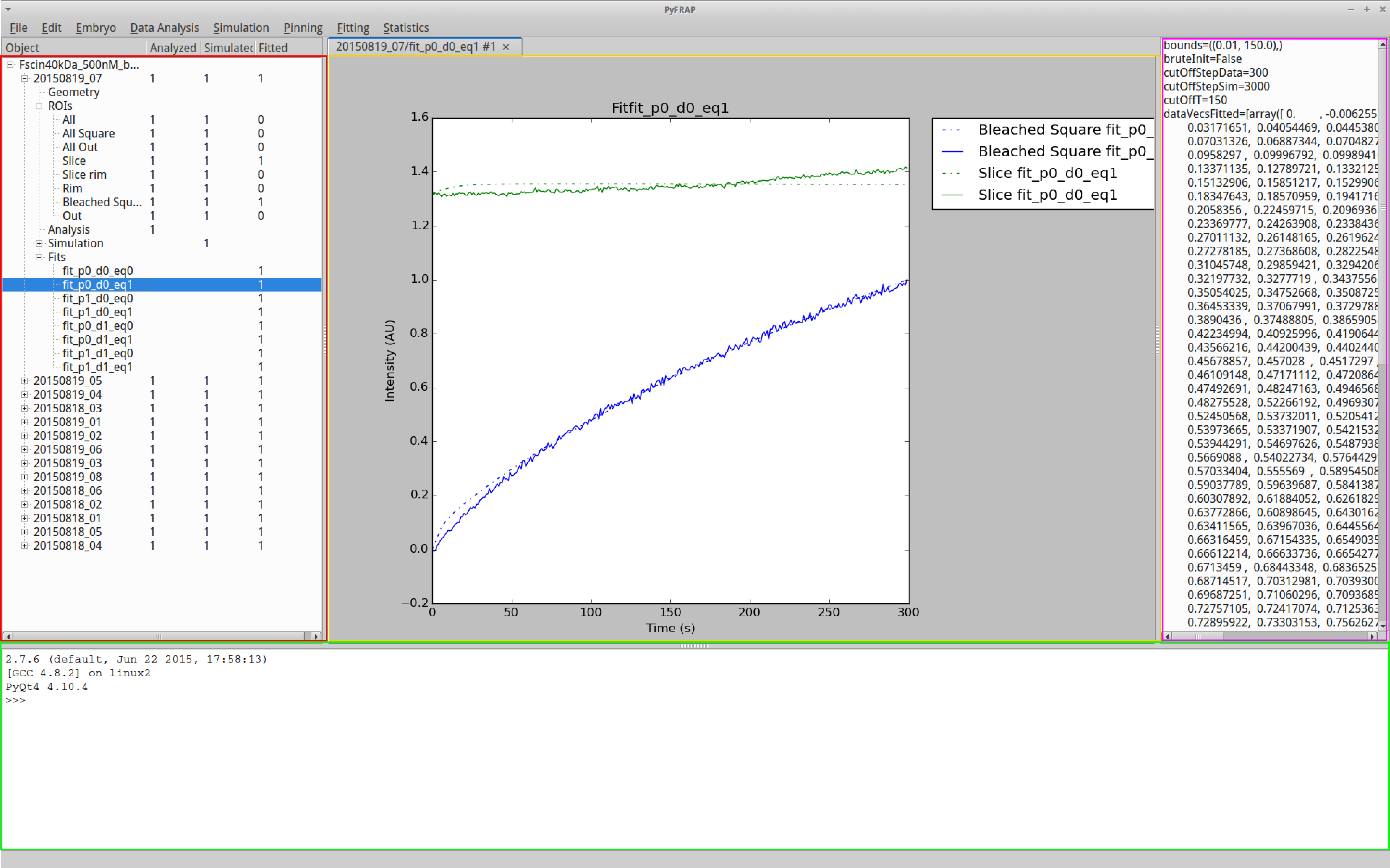
The PyFRAP GUI is divided into four main parts:

• Highlighted in red on the left is the object bar. All currently loaded projects and experiments are listed here. This makes it easy to quickly navigate between different experiments.
• On the opposite side indicated in pink is the property bar. This bar displays the properties of the currently selected object in the object bar. This makes it possible to quickly inspect object properties.
• In the center in yellow is the plot tab panel. All plots within PyFRAP open a new tab in the plot tab panel, making it easy for you to switch and compare between plots.
• In the bottom of the PyFRAP window (green) is the console. The console is a fully running Python console. This gives you as a PyFRAP user full customizabilty. You can access all of PyFRAPs modules plus any other Python module directly, run scripts, or check object properties.

Analyzing a FRAP dataset with PyFRAP

Analyzing FRAP data with PyFRAP is straightforward, however requires the user to follow an exact work flow. The PyFRAP standard work flow can be summarized in the following steps:

1. Setup project: Create the necessary PyFRAP data structure, tell PyFRAP where the image data is located and set all important parameters of the experiment.
2. Image analysis: Analyze the image data.
3. Simulation: Peform a reference simulation of the FRAP experiment.
4. Fitting: Fit the reference simulation by scaling to the analyzed image data.

Here we go through a standard work flow using a sample FRAP dataset of an experiment with injected Squint-GFP mRNA in a living zebrafish embryo. The dataset can be obtained from here. Download the test dataset and unzip it to the location of your preference. Make sure that you do not have any spaces in the filepath.

Step 0: Know your data

This is the most crucial step, and correct data analysis is largely based on understanding the underlying data. Before you start analyzing data, make sure that you have a good understanding of all known experimental aspects

• Depth of imaging,
• Possible underlying reaction kinetics,
• Geometry of the sample,
• Underlying diffusion dynamics,
• Time scale of experiment,
• Illumination inhomogeneities, and
• Microscope details.

It goes without saying that PyFRAP's analysis will be based on your knowledge and assumptions of the data and it is thus important to clearly note these down and provide them with the analyzed data.

In this tutorial we use a FRAP dataset of the morphogen Squint attached to GFP in a living zebrafish embryo at dome stage. The Squint-GFP signal is produced from injected mRNA encoding the fusion protein. Since the FRAP experiment is conducted over 50 minutes, a decent portion of the recovery observed during the experiment stems from newly produced proteins during the experiment. Moreover, we know that the experiment is conducted in a dome stage zebrafish embryo at roughly 40 microns depth. We will mention when these details become important during the analysis in the following tutorial.

Step 1: Setup Project

PyFRAP comes with a hierarchical data structure. The root structure are molecules. molecule objects collect FRAP experiments, called embryos, and allow you to do statistical comparisons between all included experiments.

To create a molecule, go to File --> New Molecule. You will then be asked to give your molecule a name, such as "sqtGFP_50pg_zebrafish".

Step 2: Launching the PyFRAP wizard

Now that we have created a new project, we can add a new experiment. If you are using PyFRAP for the first time, we highly recommend using the PyFRAP wizard. This wizard will guide you through setting up a proper FRAP analysis, to the actual analysis, simulation and fitting. To make use of the wizard, go to Edit --> PyFRAP Wizard. We will now guide you through the steps of the wizard.

Step 3: Creating an embryo object from microscope data

Step 3.1: Importing microscope data

The first dialog that appears lets you choose between two options:

• Create Embryo from Microscope Data: Select this option if your data is still in form of mircoscope files, such as .czi.
• Create Embryo from already prepared Data: Select this option if your data is already exported in single .tif files and sorted in the right folder structure.

Our test dataset is in the .czi format, so we will select the first option. This will launch the following dialog:

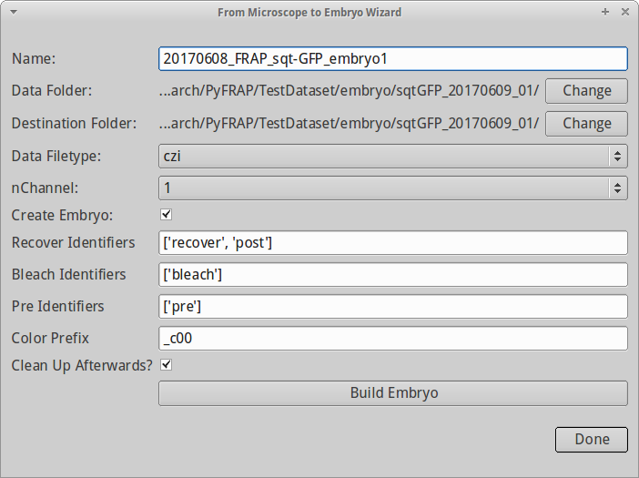
The dialog has the following fields:

• Name: Name of the embryo (your dataset); for the test data, type the base name 20170608_FRAP_sqt-GFP_embryo1
• Data Filetype: This is the type of data. We will select .czi files. **You have to do this before you select Data Folder **.
• Data Folder: This is the location of your data, e.g. the folder containing your .czi files. Click on Change to navigate there.
• Destination Folder: PyFRAP will automatically create a folder structure in a given folder. By default, it will use the same folder as Data Folder for it. For now, we do not change this.
• nChannel: The channel of interest. If you recorded multiple channels in your .czi file, select the correct one. For now, we leave it at 1.
• Create Embryo: Create an embryo object on the fly? We leave this one checked. This option is only useful for bigger projects launched from scripts.
• Recover identifiers, Bleach identifiers, Pre identifiers: You need to tell PyFRAP how it is supposed to distinguish between the recovery data, the bleaching data and the pre-bleaching data. PyFRAP will automatically find the right file if you provide him with a list of keywords that help him identify the right file based on the filename. So, for instance, if your imaging data of the recovery process contains the word recover, then all .tif files produced by this dialog will be sorted in the recover folder and be treated as recovery data in the further process. For now, we do not change any of them.
• Clean up afterwards: Clean up in the folder structure, i.e. delete all temporarily created files and folders.

Now click Build Embryo. PyFRAP now calls Fiji (ImageJ) to export FRAP data from the .czi files and sort them in the right folder structure. Your terminal might show some output by Fiji. When PyFRAP is done, click Done.

Step 3.2: The Embryo Dialog

After exporting and sorting the data, the embryo dialog will pop up. Here we can define the most elementary properties of our experiment, such as

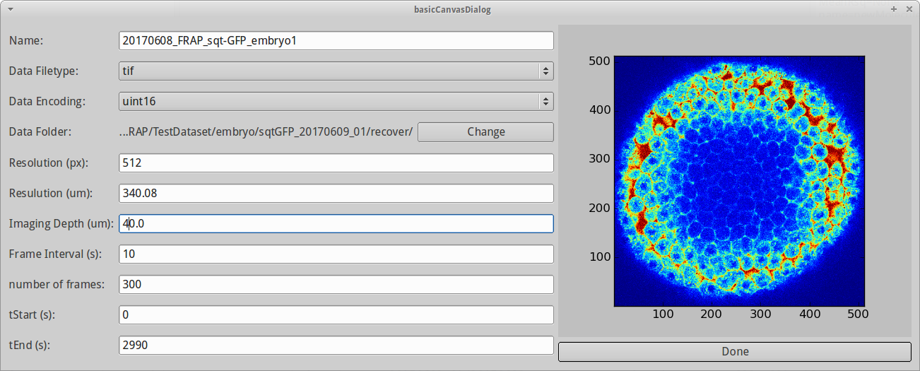
• Name: Name of the experiment
• Data Filetype: The data filetype. Right now only .tif is supported.
• Data Encoding: The encoding of the data. Can be either 16bit (uint16) or 8bit (8bit). Our example dataset is 16bit.
• Data Folder: Folder containing image files of the FRAP experiment. Since we used to microscope file extraction wizard, it is already set.
• Resolution (px): Pixel dimension in pixel. We generally assume 512x512 pixels.
• Resolution (um): Pixel dimension in microns. Here we enter 340.08.
• Imaging depth (um): The depth at which we imaged. 40 microns is a good approximation for our test data set.
• Frame interval (s): The time interval between consecutive images in seconds. For our test data set, this is 10.
• Number of frames: Number of images. Normally this gets automatically adjusted by the number of files in the recover folder.
• tStart (s): Start time of experiment. We leave that at 0.
• tEnd (s): End time of experiment. Automatically gets adjusted using nFrames, tStart and frame interval.

Note that selecting a new data folder will automatically adjust the number of frames and the time the experiment ended.

When you are done with adjusting all settings, click Done.

Step 4: Setup Geometry

One of PyFRAP's strengths is that it allows analyzing FRAP experiments in complex 3D geometries. PyFRAP comes with a few presets, but is not limited to these. For custom geometries and more fancy geometry editing, please refer to Meshing.

Step 4.1: Select Geometry

A new dialog pops up and lets you select between different geometry presets. Since the sample dataset was conducted in a zebrafish embryo at dome stage, we choose the zebraFishDomeStage. Click Done.

Step 4.2 Edit Geometry

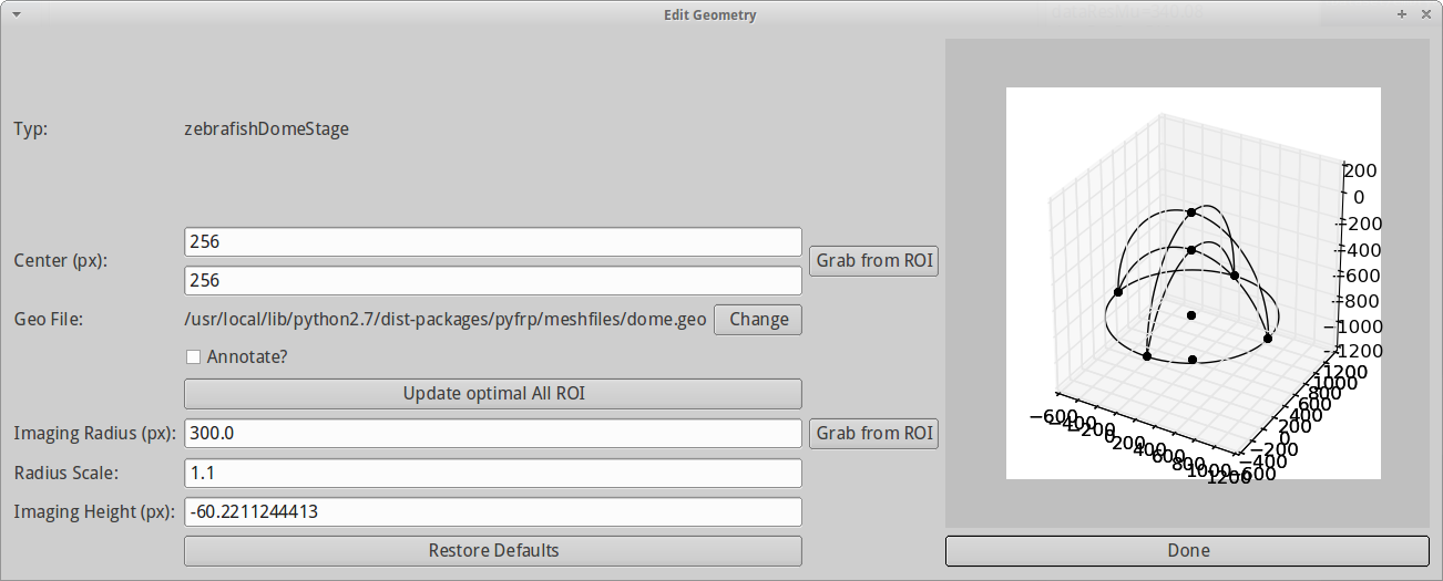
After selecting a geometry, we can define the parameters crucial to the geometry in the Edit Geometry dialog. The dialog shows your current geometry on the right-hand side and updates it as soon as you do changes on the left-hand side. Note that this can be slightly slow when geometries become complicated. PyFRAP takes your settings from the Step 3.2 and already adjusts most of the necessary settings, such as imaging height. For now, we do not have to do any changes, however, in detail, you can do the following settings

• Center (px): x- and y-coordinate of the center of your geometry (by default (256,256)). Leave unchanged.
• Geo File: Path to your current geometry (.geo) file. Leave unchanged.
• Annotate: Annotates the plot on the right hand side with the specific identifiers for each geometrical element.
• Update optimal All ROI: For later use (don't activate).
• Imaging Radius (px): Radius of the embryo in imaging depth in pixels. Leave unchanged.
• Radius Scale: Scaling between radii of the two half spheres. Leave unchanged.
• Imaging Height (px): The height at which we imaged (automatically set from imaging depth input from Step 3.2).

PyFRAP then automatically computes the dome geometry. For details, please have a look at zebrafish dome stage API.

Click Done.

Step 5: Setup ROIs

PyFRAP allows you to define arbitrary ROIs in which you can evaluate the intensities of the experiment both in the image analysis and simulation. PyFRAP comes with different wizards that allow you to setup different default sets of ROIs. If you want to read more about ROIs, please refer to the ROIs section.

After you have created the embryo's geometry, a new dialog will pop up presenting you with three options of ROI creation.

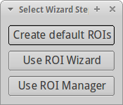
The three options are

• Create default ROIs: Simplest way to create a default set of ROIs.
• Use ROI Wizard: Creates the same set of ROIs as default ROIs, but lets you choose their dimensions more exactly.
• Use ROI Manager: Opens the ROI manager. The ROI Manager allows for the creation of arbitrary sets of ROIs.

Please refer to the ROIs section for more detail about the three options. Note that you can add, remove and edit all ROIs later using the ROI Manager.

For now, we choose Create default ROIs. This opens a new dialog showing the first post-bleach image of our dataset.

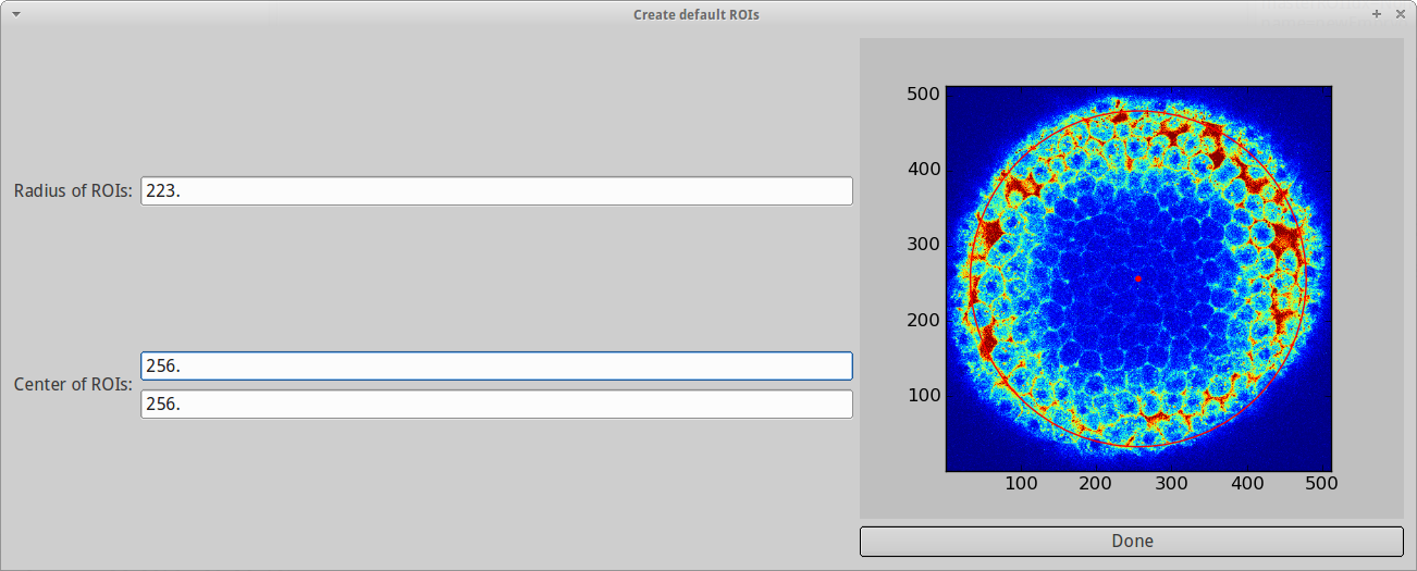
By left-clicking on the image we can select a center of a circle. Another left-click will define the radius of the circle. Right-clicking will undo the previous step. One can then fine tune the selection using keyboard shortcuts: The arrow keys allow you to move the center, and thus the circle in the respective region, and Ctrl+Up/Down increases/decreases the radius. You can also set the parameters in the text fields on the left hand side of the dialog. For our dataset, we choose a center of (256px,256px) and a radius of roughly 223px.

When clicking done, this will create a set of ROIs. The three most important of which are:

• Slice: Your complete sample in the imaging slice.
• Bleached ROI: The ROI covering the bleached zone.
• rim: A rim at the edge of the embryo, allowing PyFRAP to estimate the "rim concentration".

For more details about these ROIs, please refer to the ROIs section.

Step 6: Adjusting the geometry

After we are done with selecting our ROIs, the geometry dialog pops up once again and lets us adjust the geometry a bit further. In the case of the zebrafish dome stage, the radius and center of the Slice ROI defines the overall geometry. Thus, we need to adjust both parameters. For this geometry, PyFRAP lets the user to grab the specific values from the previously defined ROIs.

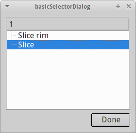
By clicking once each on the two buttons Grab from ROI and selecting Slice each time, we tell PyFRAP to use the center and radius of the Slice for the computation of the overall geometry.

Click Done.

Step 7: Mesh settings

The next step is generating a mesh. Meshes are necessary to discretize the 3-dimensional space for the reaction-diffusion simulations carried out later. Choosing the right mesh size and properties is not straightforward and will require experience. If the mesh is too coarse ( volSize too high), PyFRAP's simulation will not accurately represent the FRAP experiment and probably contain multiple numerical errors. In principle, there is no such thing as a too dense mesh - however, the denser the mesh, the longer the simulation will take and, depending on the computer you are running PyFRAP with, eventually crash.

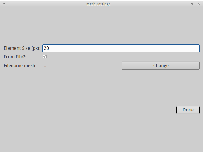
For now we choose a mesh element size of 17. This should be dense enough to approximate the FRAP experiment well while keeping the mesh at a reasonable size.

We ignore all other fields and click Done. Meshing will take a few seconds and in the end provide us with an output of the current mesh statistics in the PyFRAP terminal.

Step 8: ROI indexing

When finishing the mesh settings, PyFRAP will start to index all ROIs. That is, PyFRAP will figure out which pixels in the images and which nodes in the mesh are lying within the specified ROIs. This can take a few seconds, depending on how fine your mesh is.

Step 9: Image analysis

PyFRAP offers several methods to correct imaging artifacts for FRAP image data, such as

• Gaussian/Median Filter for smoothing/denoising
• Imaging irregularity correction via prebleach image or flattening dataset
• Background substraction
• Reduction onto quadrant (experimental!)

Since our dataset does not suffer from uneven imaging, we will only apply a median filter with radius 5 to denoise and smoothen our dataset to avoid numerical singularities during the simulation step. If you want to know more about the analysis options and its applications and implications, please refer to our original publication or the analysis section.

Pressing Done will launch the image analysis. Depending on the amount of images being analyzed and the number of manipluations applied, this can take up to a few minutes.

Step 10: Simulation

Now that we have analyzed the image data, we can simulate the same experiment. Again, finding the perfect settings of the simulation may take some time and requires experience and most of all knowledge of what you are measuring. You can set the following parameters:

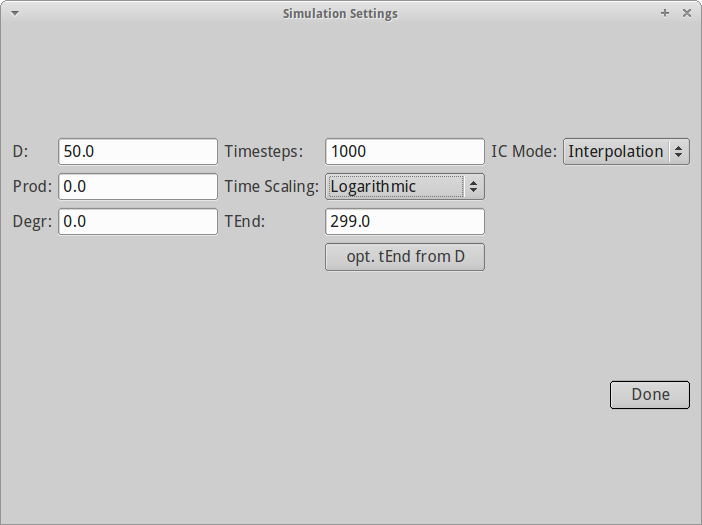
• Diffusion rate D (px^2/s)
• Production (keep at 0.)
• Degradation (keep at 0.)
• Number of simulation steps (keep it at least roughly 5 times more than the number of images you have)
• Time stepping (linear/logarithmic)
• Application of initial conditions (interpolation generally makes most sense)

For our test dataset, we use a diffusion coefficient of 50 and 1000 linear simulation time steps.

Pressing Done will launch the simulation. Depending on how fine your mesh is and how many steps you are doing, this can take again a few minutes.

Step 11: Fitting

Step 11.1: Setting up the fit

When the simulation is done, we bring data and simulation together by fitting the simulation to the data. A new dialog opens with a multitude of options, such as:

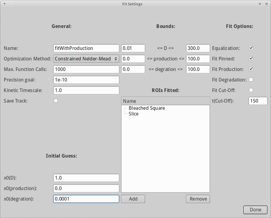
• Name of fit (makes it easier to distinguish between results).
• Optimization algorithm used.
• Lower and upper bounds for diffusion, production and degradation.
• Initial guess for all parameters.
• Which ROI to be used for fitting (generally we want to use the one that describes the bleached region best).
• Fit production/degradation?
• Pin simulation and analysis results between 0 and 1?
• Use equalization to account for changing levels in fluorescence/immobile fraction.

First, we have to select the ROIs that we consider for fitting. Since our data involves production, the pure recovery curve of the bleached region does not necessarily reveal both production and diffusion. Thus we select both Slice and Bleached Square for fitting by clicking on Add on the bottom of the dialog.

When both ROIs are added, we also need to tell PyFRAP which reaction kinetics it should consider. Since the Squint-GFP molecules are constantly produced from injected mRNA, we will select Fit Production. Also, we select Equalization and Fit Pinned to account for an immobile fraction. It is good to try out different initial guesses for D to avoid getting stuck in local minima during optimization, but for now we leave x0(D) = 10.

Moreover, we know that the degradation rate of Squint is roughly 0.0001 1/s (Müller et al. 2012). We can thus enter 0.0001 in the field x0(degr). Since we did not select Fit Degradation, this value will be kept fix during the fitting progess. In general, if the parameter is fixed ( Fit Production or Fit Degradation unchecked), PyFRAP will use the values provided via x0 as fixed. Otherwise, the values given in x0 serve as initial guesses and are subsequently varied during the fitting progress.

For the optimization method we choose Constrained Nelder-Mead.

Step 11.2: Pinning

Pressing Done will start the fitting. Since we selected fit pinned, the pinning dialog will open. We are presented with several options, mainly

• Use Min. Value for Background: Use the minimum value of the background ROI for background substraction.
• Use Max. Value for Normalization: Use the maximum value of the norm ROI for normalization.
• Show Debugging Output: Shows debugging output and plots.
• ROI for Background Calculation: ROI used for background calculation. In our case this is Bleached Square. Note that this has nothing to do with background subtraction during image analysis.
• ROI for Norm Calculation: ROI used for norm calculation. In our case this is Slice.
• Switch Threshold: Threshold at which PyFRAP overwrites the pinning settings to avoid negative concentrations.
• Pin simulation separately: Use different pinning values for analysis and simulation.

If you selected the default ROIs earlier, the default options set in this dialog will lead to good results for our test data. However, again, experience and knowledge of your FRAP experiment is key to successful FRAP analysis.

Click Done.

If we are done with fitting, go to Fitting --> Print fit results to get an output of your FRAP results. The parameter DOptMu describes the rate of diffusion in um^2/s obtained from your PyFRAP analysis. Going to Fitting -> Plotting -> Plot Fit will result in a plot like this:

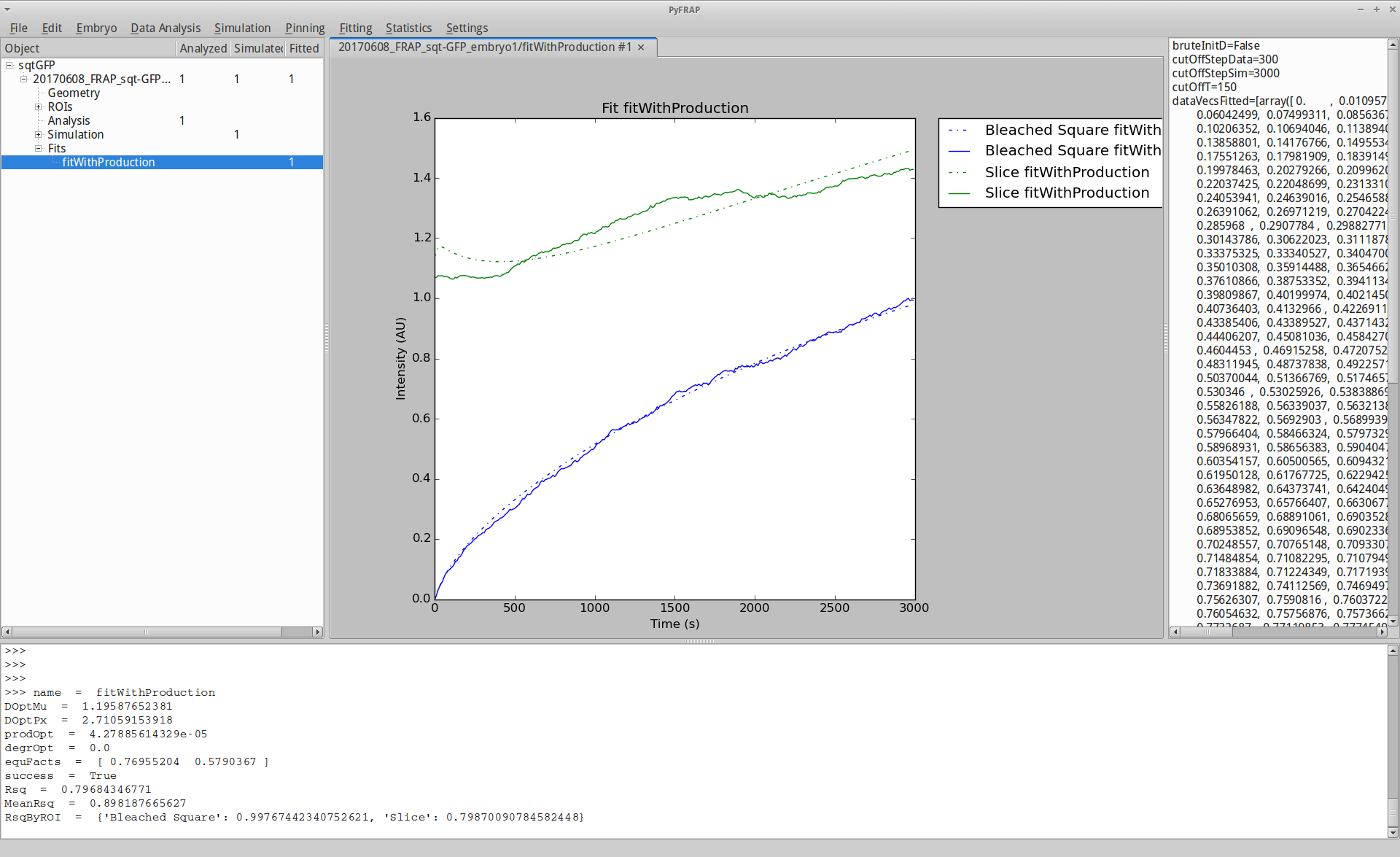
You have now analyzed your first FRAP dataset with PyFRAP. For further information and advanced options, please refer to the Wiki.