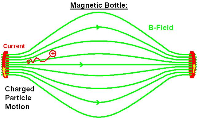
A magnetic bottle is two magnetic mirrors placed close together. For example, two parallel coils separated by a small distance, carrying the same current in the same direction will produce a magnetic bottle between them. Unlike the full mirror machine which typically had many large rings of current surrounding the middle of the magnetic field, the bottle typically has just two rings of current. Particles near either end of the bottle experience a magnetic force towards the center of the region; particles with appropriate speeds spiral repeatedly from one end of the region to the other and back. Magnetic bottles can be used to temporarily trap charged particles. It is easier to trap electrons than ions, because electrons are so much lighter This technique is used to confine very hot plasmas with temperatures of the order of 106 K.
The math equations below are written by latex. You can see a more concise version here
We can get the magnetic field which is generared by a coil(at the origin of the coordinate) by integrating
\begin{equation}
\begin{cases}
        B_{x0}(x,y,z)=\int_0^{2 \pi} \frac{Rzcos \phi}{(x^2+y^2+z^2+R^2-2xRcos \phi-2yRsin \phi)^{3/2}} d\phi\\
        B_{y0}(x,y,z)=\int_0^{2 \pi} \frac{Rzsin \phi}{(x^2+y^2+z^2+R^2-2xRcos \phi-2yRsin \phi)^{3/2}} d\phi\\
        B_{z0}(x,y,z)=\int_0^{2 \pi} \frac{R(R-xcos\phi-ysin\phi)}{(x^2+y^2+z^2+R^2-2xRcos \phi-2yRsin \phi)^{3/2}} d\phi
\end{cases}
\end{equation}
Then we can get the magnetic field of a magnetic bottle (two coils) by a transformation
 \begin{equation}
 \begin{cases}
        B_{x}(x,y,z)=B_{x0}(x,y,z-d/2)+B_{x0}(x,y,z+d/2)\\
        B_{y}(x,y,z)=B_{y0}(x,y,z-d/2)+B_{y0}(x,y,z+d/2)\\
        B_{z}(x,y,z)=B_{z0}(x,y,z-d/2)+B_{z0}(x,y,z+d/2)
 \end{cases}
 \end{equation}
d in these equations means the distance between two coils.
Calculate the trace of an electron in a magnetic bottle by solving odes(newton equation and Lorentz force)
According to the Newton equation and Lorentz force equation
\begin{equation}
\begin{cases}
    F=ma\\
    F_{Lorentz}=qv \times x
\end{cases}
\end{equation}
Then we can get the equation,
\begin{equation}
    qv \times x=ma
\end{equation}
Then we need to solve the second order Ordinary Differential Equations, because we study this problem in 3D.
\begin{equation}
    \begin{cases}
        x''=-\frac{m}{q}(y'Bz(x,y,z)-z'By(x,y,z))\\
        y''=-\frac{m}{q}(z'Bx(x,y,z)-x'Bz(x,y,z))\\
        z''=-\frac{m}{q}(x'By(x,y,z)-y'Bx(x,y,z))
    \end{cases}
\end{equation}
We transfer the them into first order Ordinary Differential Equations,
\begin{equation}
    \begin{cases}
        vx'=-sc(vy*Bz(x,y,z)-vz*By(x,y,z))\\
        vy'=-sc(vz*Bx(x,y,z)-vx*Bz(x,y,z))\\
        vz'=-sc(vx*By(x,y,z)-vy*Bx(x,y,z))\\
        x'=vx\\
        y'=vy\\
        z'=vz
    \end{cases}
\end{equation}
Its intial values are
\begin{equation}
    \begin{cases}
        vx(0)=0\\
        vy(0)=0\\
        vz(0)=0.15e6\\
        x(0)=0\\
        y(0)=0.78R\\
        z(0)=-0.75d
    \end{cases}
\end{equation}
Mathematica is a powerful mathematic and physics software. It can realize this program by very short code and its graphics in 3D and animation in 3D are cool, but its efficiency is really low.
SetDirectory[NotebookDirectory[]];

Bx0[x_, y_, z_] := NIntegrate[
   ( R z Cos[\[CurlyPhi]])/(x^2 + y^2 + z^2 + R^2 -
     2 x R Cos[\[CurlyPhi]] - 2 y R Sin[\[CurlyPhi]])^(3/2),
   {\[CurlyPhi], 0, 2 \[Pi]}, MaxRecursion -> 12];
By0[x_, y_, z_] := NIntegrate[
   ( R z Sin[\[CurlyPhi]])/(x^2 + y^2 + z^2 + R^2 -
     2 x R Cos[\[CurlyPhi]] - 2 y R Sin[\[CurlyPhi]])^(3/2),
   {\[CurlyPhi], 0, 2 \[Pi]}, MaxRecursion -> 12];
Bz0[x_, y_, z_] := NIntegrate[
   ( R (R - x Cos[\[CurlyPhi]] - y Sin[\[CurlyPhi]]))/(x^2 + y^2 +
     z^2 + R^2 - 2 x R Cos[\[CurlyPhi]] - 2 y R Sin[\[CurlyPhi]])^(
   3/2),
   {\[CurlyPhi], 0, 2 \[Pi]}, MaxRecursion -> 12];
Bx[x_, y_, z_] := Bx0[x, y, z - d/2] + Bx0[x, y, z + d/2];
By[x_, y_, z_] := By0[x, y, z - d/2] + By0[x, y, z + d/2];
Bz[x_, y_, z_] := Bz0[x, y, z - d/2] + Bz0[x, y, z + d/2];
R = 1.0; d = 2 R; n = 50;
data1 = {};
Do[
 Do[
  Do[AppendTo[data1, {(3 R)/n i, (3 R)/n j, (2 d)/n k,
     Bx[(3 R)/n i, (3 R)/n j, (2 d)/n k]}],
   {i, -n/2, n/2}],
  {j, -n/2, n/2}],
 {k, -n/2, n/2}]
Bx = Interpolation[data1];
Bx >> "Bx50";
data2 = {};
Do[
 Do[
  Do[AppendTo[data2, {(3 R)/n i, (3 R)/n j, (2 d)/n k,
     By[(3 R)/n i, (3 R)/n j, (2 d)/n k]}],
   {i, -n/2, n/2}],
  {j, -n/2, n/2}],
 {k, -n/2, n/2}]
By = Interpolation[data2];
By >> "By50";
data3 = {};
Do[
 Do[
  Do[AppendTo[data3, {(3 R)/n i, (3 R)/n j, (2 d)/n k,
     Bz[(3 R)/n i, (3 R)/n j, (2 d)/n k]}],
   {i, -n/2, n/2}],
  {j, -n/2, n/2}],
 {k, -n/2, n/2}]
Bz = Interpolation[data3];
Bz >> "Bz50";

SetDirectory[NotebookDirectory[]];
R = 1; d = 2 R;
sc = 1.75851*10^11*0.35*10^-5; time = 60 10^-6;
<< "Bx50";
Bx = %;
<< "By50";
By = %;
<< "Bz50";
Bz = %;
equ = {x''[t] == -sc (y'[t] Bz[x[t], y[t], z[t]] -
       z'[t] By[x[t], y[t], z[t]]),
   y''[t] == -sc (z'[t] Bx[x[t], y[t], z[t]] -
       x'[t] Bz[x[t], y[t], z[t]]),
   z''[t] == -sc (x'[t] By[x[t], y[t], z[t]] -
       y'[t] Bx[x[t], y[t], z[t]]),
   x[0] == 0, x'[0] == 0, y[0] == 0, y'[0] == 0.3 10^6,
   z[0] == 0, z'[0] == 0.15 10^6};
s = NDSolve[equ, {x, y, z}, {t, 0, time}]
{x, y, z} = {x, y, z} /. s[[1]];
Manipulate[ParametricPlot3D[{x[t], y[t], z[t]},
  {t, 0, t0}, Ticks -> None, AxesStyle -> Thin, Axes -> True,
  AxesLabel -> {"x", "y", "z"},
  PlotStyle -> {Thin, Black}, AspectRatio -> 2,
  PlotRange -> {{- 0.3 d, 0.3 d}, {-0.3 d, 0.3 d}, {-0.75 d,
     0.75 d}}], {t0, 0.001 time, time}]
This picture shows the configuration of a magnetic bottle. The grey vectors represent the magnetic field. Two yellow rings means two coils with the same current. Red lines presents the trace of an electron. The blue arrow means the initial position and velocity of the electron.

This gif shows the movement of an electron in a magnetic bottle.(Notice the two coils actually are on the z axle, which is different from the picture above. You can see this gif by rotating your head by 90 degree)

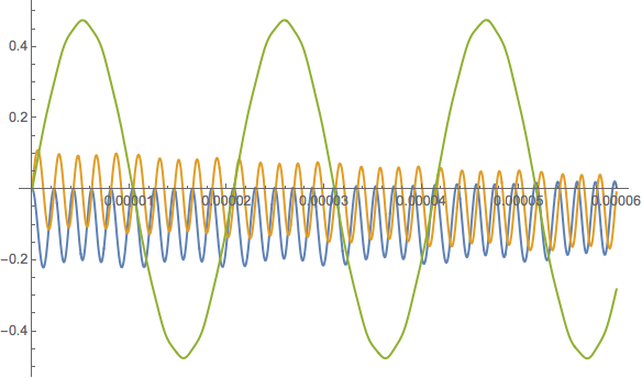
This figure shows the x,y,z coordinate changing with time.
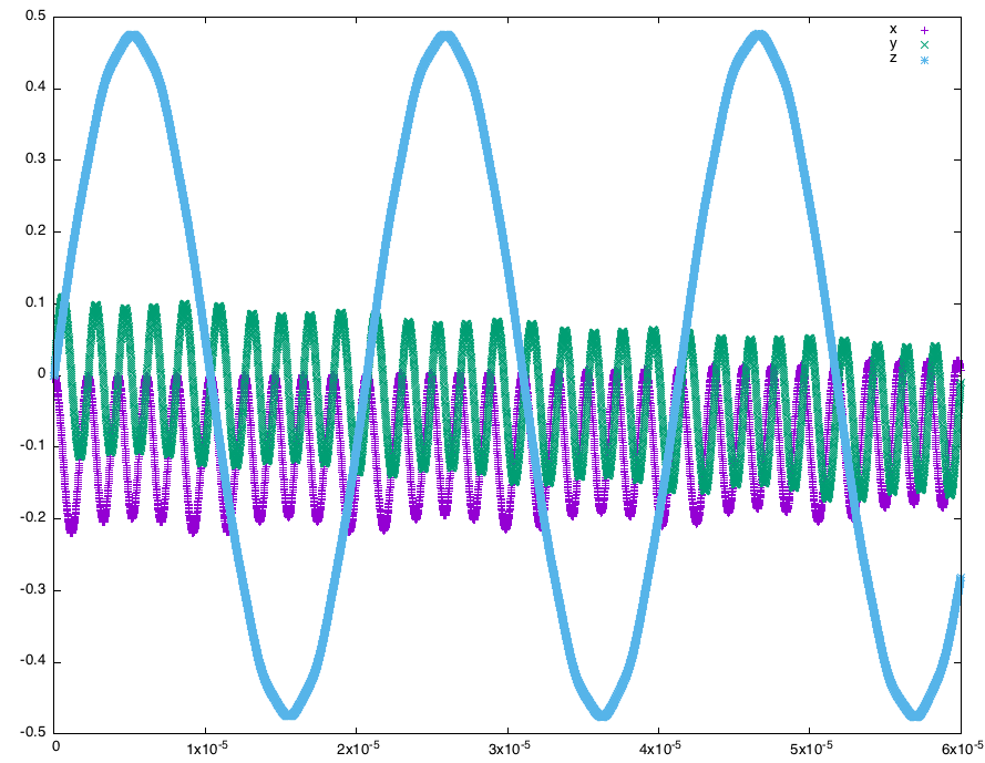
Although C is much more complicate than Mathematica and its code is much longer, its efficiency is much higher and OpenGl is good at graphics and animation.
This figure shows the x,y,z coordinate changing with time, which is almost same to the one calculated by Mathematica.
-
double click the magnetic_mirror.exe (do not delete the "glut.lib","glut.h",etc in the folder)
-
input the initial values
-
press 'a' to start the animation in the 'plasma' window (not the terminal window)
-
press 's' to stop the animation
-
press the left button and drag it to change the view
In this program, you can input the ratio of velocity y and velocity z in the terminal window. When this ratio is too small(i.e ratio<1), the electron will escape from the magnetic mirror. Actually, many parameters can be changed. For instance, the initial velocity and position of the electron can also be changed, which will cause different electron trace. You even can change the configuration of the magnetic mirror (i.e the ratio of the distance of the two coils and the radius of the coil), which can change the magnetic field line and the trace. However, I fix these parameters in case the parameters you input do not have correct physical meanings.