Mention possible filters in radon_transform -> filtered-back-projection

[kolibril13]

Description

As this section https://scikit-image.org/docs/dev/auto_examples/transform/plot_radon_transform.html#reconstruction-with-the-filtered-back-projection-fbp explains that one can use filters, I think it would be nice to explicitly mention these filters.
Further, it might be nice to show an image of the filters, e.g. like this:

which was produced by this code:

import numpy as np
import matplotlib.pylab as plt
from scipy.fftpack import fft

def frequency_response(size,filter_name):
    
    n = np.concatenate((np.arange(1, size / 2 + 1, 2, dtype=int),
                        np.arange(size / 2 - 1, 0, -2, dtype=int)))
    f = np.zeros(size)
    f[0] = 0.25
    f[1::2] = -1 / (np.pi * n) ** 2

    # Computing the ramp filter from the fourier transform of its
    # frequency domain representation lessens artifacts and removes a
    # small bias as explained in [1], Chap 3. Equation 61
    fourier_filter = 2 * np.real(fft(f))         # ramp filter
    if filter_name == "ramp":
        pass
    elif filter_name == "shepp-logan":
        # Start from first element to avoid divide by zero
        omega = np.pi * np.fft.fftfreq(size)[1:]
        fourier_filter[1:] *= np.sin(omega) / omega
    elif filter_name == "cosine":
        freq = np.linspace(0, np.pi, size, endpoint=False)
        cosine_filter = np.fft.fftshift(np.sin(freq))
        fourier_filter *= cosine_filter
    elif filter_name == "hamming":
        fourier_filter *= np.fft.fftshift(np.hamming(size))
    elif filter_name == "hann":
        fourier_filter *= np.fft.fftshift(np.hanning(size))
    elif filter_name is None:
        fourier_filter[:] = 1

    return fourier_filter[:, np.newaxis]



filters = ['ramp', 'shepp-logan', 'cosine', 'hamming', 'hann']

for ix, f in enumerate(filters):
    response = frequency_response(2000,f)
    plt.plot(response, label= f)
plt.legend()
plt.show()

the code is basically this function:

scikit-image/skimage/transform/radon_transform.py

Lines 128 to 181 in 944760c

	def _get_fourier_filter(size, filter_name):
	"""Construct the Fourier filter.
	This computation lessens artifacts and removes a small bias as
	explained in [1], Chap 3. Equation 61.
	Parameters
	----------
	size: int
	filter size. Must be even.
	filter_name: str
	Filter used in frequency domain filtering. Filters available:
	ramp, shepp-logan, cosine, hamming, hann. Assign None to use
	no filter.
	Returns
	-------
	fourier_filter: ndarray
	The computed Fourier filter.
	References
	----------
	.. [1] AC Kak, M Slaney, "Principles of Computerized Tomographic
	Imaging", IEEE Press 1988.
	"""
	n = np.concatenate((np.arange(1, size / 2 + 1, 2, dtype=int),
	np.arange(size / 2 - 1, 0, -2, dtype=int)))
	f = np.zeros(size)
	f[0] = 0.25
	f[1::2] = -1 / (np.pi * n) ** 2
	# Computing the ramp filter from the fourier transform of its
	# frequency domain representation lessens artifacts and removes a
	# small bias as explained in [1], Chap 3. Equation 61
	fourier_filter = 2 * np.real(fft(f)) # ramp filter
	if filter_name == "ramp":
	pass
	elif filter_name == "shepp-logan":
	# Start from first element to avoid divide by zero
	omega = np.pi * fftmodule.fftfreq(size)[1:]
	fourier_filter[1:] *= np.sin(omega) / omega
	elif filter_name == "cosine":
	freq = np.linspace(0, np.pi, size, endpoint=False)
	cosine_filter = fftmodule.fftshift(np.sin(freq))
	fourier_filter *= cosine_filter
	elif filter_name == "hamming":
	fourier_filter *= fftmodule.fftshift(np.hamming(size))
	elif filter_name == "hann":
	fourier_filter *= fftmodule.fftshift(np.hanning(size))
	elif filter_name is None:
	fourier_filter[:] = 1
	return fourier_filter[:, np.newaxis]

Checklist

• Docstrings for all functions
• Gallery example in ./doc/examples (new features only)
• Benchmark in ./benchmarks, if your changes aren't covered by an
  existing benchmark
• Unit tests
• Clean style in the spirit of PEP8

For reviewers

• Check that the PR title is short, concise, and will make sense 1 year
  later.
• Check that new functions are imported in corresponding __init__.py.
• Check that new features, API changes, and deprecations are mentioned in
  doc/release/release_dev.rst.

[pep8speaks]

Hello @kolibril13! Thanks for updating this PR. We checked the lines you've touched for PEP 8 issues, and found:

• In the file doc/examples/transform/plot_radon_transform.py:

Line 104:1: E402 module level import not at top of file
Line 105:1: E402 module level import not at top of file

Comment last updated at 2021-03-23 16:23:00 UTC

[rfezzani]

Excellent suggestion @kolibril13, thank you! The figure you generated is also nice, you can add it to your PR 😉

[kolibril13]

Thanks for the feedback!
Regarding the way to include the image I see three approaches:

1.

Adding the _get_fourier_filter to __all__ and then adding a short script:

filters = ['ramp', 'shepp-logan', 'cosine', 'hamming', 'hann']
for ix, f in enumerate(filters):
    response = frequency_response(2000,f)
    plt.plot(response, label= f)
plt.legend()
plt.xlabel("Position in Pixel")
plt.show()

But that would make changes to the core library, which might not be wanted (although I think having access to the frequency_response function might be useful in other cases as well.)

2.

3. Copying the complete code from get_fourier_filter to this example, like this:

import numpy as np
import matplotlib.pylab as plt
from scipy.fftpack import fft

def frequency_response(size,filter_name):
    
    n = np.concatenate((np.arange(1, size / 2 + 1, 2, dtype=int),
                        np.arange(size / 2 - 1, 0, -2, dtype=int)))
    f = np.zeros(size)
    f[0] = 0.25
    f[1::2] = -1 / (np.pi * n) ** 2

    # Computing the ramp filter from the fourier transform of its
    # frequency domain representation lessens artifacts and removes a
    # small bias as explained in [1], Chap 3. Equation 61
    fourier_filter = 2 * np.real(fft(f))         # ramp filter
    if filter_name == "ramp":
        pass
    elif filter_name == "shepp-logan":
        # Start from first element to avoid divide by zero
        omega = np.pi * np.fft.fftfreq(size)[1:]
        fourier_filter[1:] *= np.sin(omega) / omega
    elif filter_name == "cosine":
        freq = np.linspace(0, np.pi, size, endpoint=False)
        cosine_filter = np.fft.fftshift(np.sin(freq))
        fourier_filter *= cosine_filter
    elif filter_name == "hamming":
        fourier_filter *= np.fft.fftshift(np.hamming(size))
    elif filter_name == "hann":
        fourier_filter *= np.fft.fftshift(np.hanning(size))
    elif filter_name is None:
        fourier_filter[:] = 1

    return fourier_filter[:, np.newaxis]



filters = ['ramp', 'shepp-logan', 'cosine', 'hamming', 'hann']

for ix, f in enumerate(filters):
    response = frequency_response(2000,f)
    plt.plot(response, label= f)
plt.legend()
plt.show()

I don't like this option too much, because it would display a lot of extra code in this section, and further, it needs to be changed when frequency_response would change in future.

3.

Adding the image as a static file here: https://github.com/kolibril13/scikit-image/tree/patch-1/doc/source/_static

[mkcor]

Hi @kolibril13,

You can readily import internal function _get_fourier_filter:

from skimage.transform.radon_transform import _get_fourier_filter

[kolibril13]

Hi @kolibril13,

You can readily import internal function _get_fourier_filter:

from skimage.transform.radon_transform import _get_fourier_filter

An elegant solution, thanks! I've now updated the pr, it is now ready for review.

[rfezzani]

Just to address PEP8 complaints 😉

[rfezzani]

Thank you @kolibril13!

[mkcor]

Approving up to the rendering suggestion I made, after looking at the rendered web page.

PS: When using the GitHub interface, note that, instead of committing them one by one, you can add several code review suggestions to a single batch and commit the latter at once. Well, here I only made one suggestion anyway. Thanks, @kolibril13!

[kolibril13]

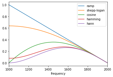
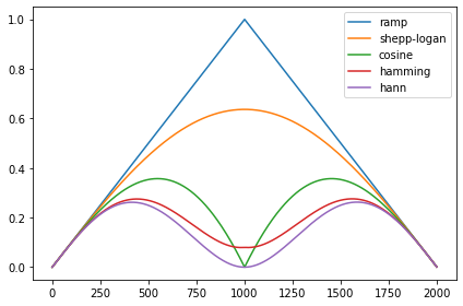
Before merging, I have one thing that seems to be a bit weird:
The frequency filters are supposed to reduce the low frequencies, hence the minimum of the filter function should be in the middle, as it can be seen for example here:

https://www.researchgate.net/figure/a-Ram-Lak-Hamming-and-Hanning-filters-in-frequency-domain-b-Ram-Lak-Hamming-and_fig1_274733291
I get the same result when I shift the x values of the filter functions by half of its total length.:

import matplotlib.pyplot as plt
from skimage.transform.radon_transform import _get_fourier_filter

filters = ["ramp", "shepp-logan", "cosine", "hamming", "hann"]
for f in filters:
    response = _get_fourier_filter(1000, f)
    response=np.roll(response, int(len(response)/2))
    plt.plot(response, label=f)
plt.legend()
plt.xlabel("frequency domain")
plt.show()

But I don't know the reason for this.
Maybe this might be related to this line, and that the Fourier transform of the image is not shifted.

scikit-image/skimage/transform/radon_transform.py

Line 291 in 944760c

projection = fft(img, axis=0) * fourier_filter

[mkcor]

Good catch, @kolibril13! I would think that the shift should happen upstream, i.e., when constructing the actual Fourier filter, so when defining function _get_fourier_filter(): fourier_filter = fftmodule.fftshift(fourier_filter) should replace

scikit-image/skimage/transform/radon_transform.py

Line 165 in a69d492

pass

and be added after

scikit-image/skimage/transform/radon_transform.py

Line 169 in a69d492

fourier_filter[1:] *= np.sin(omega) / omega

Let me look at the existing tests...

[mkcor]

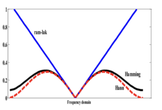
Hi @kolibril13,

I checked and, actually, the code is correct. The ramp filter, which is the default filter, is a high-pass filter: Its value is zero (minimum) at zero (lowest frequency). In the picture you attached, the middle value on the x-axis must be zero.

Please refer to these references for more details:

• https://www.mathworks.com/help/images/ref/iradon.html
• https://homepages.inf.ed.ac.uk/rbf/CVonline/LOCAL_COPIES/AV0405/HAYDEN/Slice_Reconstruction.html

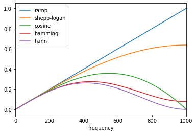
Specify the frequency range when displaying the plot:

import matplotlib.pyplot as plt
from skimage.transform.radon_transform import _get_fourier_filter

filters = ['ramp', 'shepp-logan', 'cosine', 'hamming', 'hann']

for ix, f in enumerate(filters):
    response = _get_fourier_filter(2000, f)
    plt.plot(response, label= f)

plt.xlim([0, 1000])
plt.xlabel('frequency')
plt.legend()
plt.show()

[kolibril13]

I checked and, actually, the code is correct. The ramp filter, which is the default filter, is a high-pass filter: Its value is zero (minimum) at zero (lowest frequency). In the picture you attached, the middle value on the x-axis must be zero.

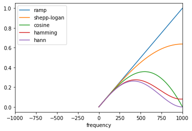
Thanks for clarifying, that sounds logical to me, and I updated the pr according to your limits with plt.xlim([0, 1000])
But still, I am confused by the range plt.xlim([1000, 2000]):

Should it not be something like this?:

import matplotlib.pyplot as plt
from skimage.transform.radon_transform import _get_fourier_filter

filters = ['ramp', 'shepp-logan', 'cosine', 'hamming', 'hann']

for ix, f in enumerate(filters):
    response = _get_fourier_filter(2000, f)
    plt.plot(response, label= f)

plt.xlim([-1000, 1000])
plt.xlabel('frequency')
plt.legend()
plt.show()

where the left side of the k-space should be filled as well?

[mkcor]

Thank you for updating the PR, @kolibril13! I just found some last minor details to fix... 😉

Should it not be something like this?
where the left side of the k-space should be filled as well?

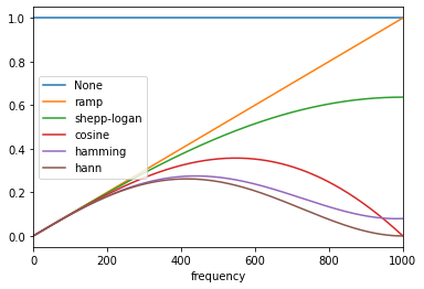
Well, it is like this! The filter is of size 2000 (cutoff frequency). So the spectrum is infinitely repeating every 2000. The ramp filter is the absolute value function on its bandwidth (see my previous reply). Since the filter is symmetric and periodic, it is enough to represent it on [0, 1000] to show all the information.

[kolibril13]

@mkcor :
Thanks for merging and your follow up pr!
I am glad I could contribute to this amazing project.

I just realized that "None" is also a filter option (

scikit-image/skimage/transform/radon_transform.py

Line 178 in 358ce87

elif filter_name is None:

) for the inverse radon, maybe one can add this for completeness, however it won't be too important.
Here would be the included idea:

import matplotlib.pyplot as plt
from skimage.transform.radon_transform import _get_fourier_filter

filters = [None,'ramp', 'shepp-logan', 'cosine', 'hamming', 'hann']

for ix, f in enumerate(filters):
    response = _get_fourier_filter(2000, f)
    if f is None:
        plt.plot(response, label="None")
    else:
        plt.plot(response, label=f)

plt.xlim([0, 1000])
plt.xlabel('frequency')
plt.legend()
plt.show()

[mkcor]

#6174 brought me back to this conversation, and I realize that

import matplotlib.pyplot as plt
from skimage.transform.radon_transform import _get_fourier_filter

filters = ['ramp', 'shepp-logan', 'cosine', 'hamming', 'hann']

for ix, f in enumerate(filters):
    response = _get_fourier_filter(2000, f)
    plt.plot(response, label= f)

plt.xlim([-1000, 1000])
plt.xlabel('frequency')
plt.legend()
plt.show()

should be it -- and, no

where the left side of the k-space should be filled as well?

the left side of the k-space should not be filled. Unlike what I wrote on March 23, 2021,

the filter is symmetric and periodic,

the filter is periodic but not symmetric: The negative half of each spectral period is set to zero (see Figure 2 (c) in https://www.gaussianwaves.com/2017/04/analytic-signal-hilbert-transform-and-fft/).