ENH:stats: Add _sf and _isf methods to kappa3

[OmarManzoor]

Reference issue

Towards: gh-17832

What does this implement/fix?

• Adds the _isf method to the Kappa3 distribution to improve its precision

Additional information

[OmarManzoor]

from scipy.stats import kappa3
from scipy.special import xlog1py, expm1
import numpy as np
import matplotlib.pyplot as plt


def _isf(q, a):
    lg = xlog1py(-a, -q)
    den = expm1(lg)
    return (a / den)**(1.0 / a)


def plot_isf():
    a = 2.0
    q = np.logspace(-30, -1, 200)
    plt.semilogx(q, kappa3.isf(q, a), label="main", ls="dashed")
    plt.semilogx(q, _isf(q, a), label="pr", ls="dotted")
    plt.legend()
    plt.title("kappa3 inverse survival function")
    plt.show()

[mdhaber]

If the new round trip test doesn't pass with this distribution, can you add an _sf?

[OmarManzoor]

If the new round trip test doesn't pass with this distribution, can you add an _sf?

I ran both test_continuous_basic and test_distributions on my local system and they seemed to pass.

[mdhaber]

Please try it again after adding a case for this distribution to the new test.

[OmarManzoor]

Please try it again after adding a case for this distribution to the new test.

You are right we need to override the _sf method. I might need a bit of time to implement that.

[OmarManzoor]

from scipy.stats import kappa3
import numpy as np
import matplotlib.pyplot as plt
from mpmath import mp
mp.dps = 200

def mpmath_sf(x, a):
    x = mp.mpf(x)
    a = mp.mpf(a)

    return mp.one - x*(a + x**a)**(-mp.one/a)


def plot_sf():
    a = 2.0
    x = np.logspace(-5, 40, 200)
    mp_values = np.array([mpmath_sf(_x, a) for _x in x], np.float64)
    plt.loglog(x, kappa3.sf(x, a), label="main", ls="dashdot")
    plt.semilogx(x, _sf(x, a), label="pr", ls="dashed")
    plt.loglog(x, mp_values, label="mpmath", ls="dotted")
    plt.legend()
    plt.title("kappa3 survival function")
    plt.show()

[mdhaber]

I thought I'd share the code I used to find these cases.

Start by defining a population of input parameters at which to test the SF and ISF functions. Hopefully, we'd have noticed already if arguments in the range 0.1 through 0.9 (e.g. kappa3.isf(0.31, 0.55)) led to inaccurate results, so the computational experiment focuses on extreme arguments. Specifically, the p-values we'll use as inputs to the ISF function are:

log_min_p = -300
log_1m_max_p = -14
p0 = np.concatenate((10**rng.uniform(log_min_p, np.log10(0.5), size=n),  # lots of points close to 0
                     1 - 10**rng.uniform(log_1m_max_p, np.log10(0.5), size=int(.05*n))))  # fewer points close to 1

The values of the shape parameter are also log-uniformly distributed:

log10_min_a = -10
log10_max_a = 10
a0 = 10**rng.uniform(log10_min_a, log10_max_a, size=len(p0))

isf is a reference implementation computed using mpmath with sufficient precision. We can then compute the values of q corresponding with the p values:

q = isf(p0, a0)

Many of these q values will have magnitude beyond the range that can be represented accurately by float64. I filter these out, so I'm left with widely distributed values of p and a that result in a float64-representable value of the ISF. In principle, then, we'd hope for our ISF implementation to be able to return an accurate result given these inputs. We can compute the relative error of our implementations (both this PR and main) against mpmath and plot a histogram. Before plotting, we clip the relative errors to the range 1e-20 to 1 since a) errors less than ~1e-16 are exactly 0 and b) we don't care about the exact error if it's greater than 1 (any amount worse than very bad is still very bad...).

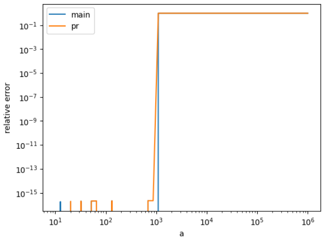
The new implementation has much lower error for this population, but you can see there are some points for which it is not accurate. We can figure out which those are by plotting the error as a function of the arguments.

So we see that large values of a for moderate values of p cause problems. Plots for the sf method show a similar story.

Note that the population we used was good at sniffing out inaccuracies, but if it is not representative of the population of arguments users will pass into the function, we can't use the histogram to conclude that the PR's implementation is better for SciPy. I don't know the answer to that question.

import numpy as np
from scipy import special as sc
from scipy import stats
from mpmath import mp
mp.dps = 1000
import matplotlib.pyplot as plt

# Reference SF
@np.vectorize
def sf(x, a):
  x, a = mp.mpf(x), mp.mpf(a)
  return mp.one - x*(a + x**a)**(-mp.one/a)

# Reference ISF
@np.vectorize
def isf(x, a):
  x, a = mp.mpf(x), mp.mpf(a)
  y = mp.one - x
  return (a/(y**-a - 1.0))**(1.0/a)

# Determine whether the value can be represented in float64
@np.vectorize
def is_float_representable(x):
  finfo = np.finfo(np.float64)
  return abs(x) > finfo.tiny and finfo.min < x < finfo.max

# Calculate the log10 of the relative error, clipping to relevant range
def log_relative_error(res, ref):
  err = abs((res - ref)/ref)
  err = err.astype(np.float64)
  # we probably don't care much about the magnitude of relative error
  # beyond this range
  err = np.clip(err, 1e-20, 1)
  return np.log10(err)

n = 1000

# Define population of arguments at which to test the ISF
log_min_p = -300
log_1m_max_p = -14
rng = np.random.default_rng(32492342965356)
p0 = np.concatenate((10**rng.uniform(log_min_p, np.log10(0.5), size=n), 
                     1 - 10**rng.uniform(log_1m_max_p, np.log10(0.5), size=int(.05*n))))
p0 = np.sort(p0)

log10_min_a = -10
log10_max_a = 10
a0 = 10**rng.uniform(log10_min_a, log10_max_a, size=len(p0))

# Compute the ISF using the reference implementation
q = isf(p0, a0)
# Filter out cases for which the result can't be represented in float64
i = is_float_representable(q)
# these are the inputs we'll use for tests of isf
a_isf = a0[i].astype(np.float64)
p_isf = p0[i].astype(np.float64)
# these are the reference values
isf_mp = q[i].astype(np.float64)

# Now we'll use the float64-representable ISF values as input to the SF
# Compute the SF using the reference implementation
sf_mp = sf(isf_mp, a_isf)
# Filter out cases for which the result can't be represented in float64
i = is_float_representable(sf_mp)
# (All should be if start with float64-representable population)
assert np.all(i)
# these are the inputs we'll use for tests of sf
a_sf = a_isf[i]
q_sf = isf_mp[i]
# these are the reference values
sf_mp = sf_mp[i]

### SF Error Histogram ###
# PR SF implementation
def _sf(x, a):
  lg = sc.xlog1py(-1.0 / a, a * x**-a)
  return -sc.expm1(lg)

# Compute and plot the SF errors
sf_pr = _sf(q_sf, a_sf)
sf_main = stats.kappa3.sf(q_sf, a_sf)

err_pr = log_relative_error(sf_pr, sf_mp)
err_main = log_relative_error(sf_main, sf_mp)

bins = np.arange(-20, 0.5, 0.5)
plt.hist(err_pr, alpha=0.5, label='PR', bins=bins)
plt.hist(err_main, alpha=0.5, label='main', bins=bins)
plt.xlabel('log10 of error')
plt.title('SF method comparison')
plt.legend()

### SF scatter plot ###
x = np.log10(q_sf)
y = np.log10(a_sf)
plt.scatter(x, y, c=err_pr)
cbar = plt.colorbar()
plt.xlabel('q')
plt.ylabel('a')
cbar.set_label('log10 of error')
plt.title('The effect of arguments on kappa.sf error (PR)')

### ISF Error Histogram ### 
def _isf(q, a):
  lg = sc.xlog1py(-a, -q)
  denom = sc.expm1(lg)
  return (a / denom)**(1.0 / a)

# Test ISF
isf_pr = _isf(p_isf, a_isf)
isf_main = stats.kappa3.isf(p_isf, a_isf)

err_pr = log_relative_error(isf_pr, isf_mp)
err_main = log_relative_error(isf_main, isf_mp)

bins = np.arange(-20, 0.5, 0.5)
plt.hist(err_pr, alpha=0.5, label='PR', bins=bins)
plt.hist(err_main, alpha=0.5, label='main', bins=bins)
plt.xlabel('log10 of error')
plt.title('ISF method comparison')
plt.legend()

### ISF Scatter Plot
x = np.log10(p_isf)
y = np.log10(a_isf)
plt.scatter(x, y, c=err_pr)
cbar = plt.colorbar()
plt.xlabel('p')
plt.ylabel('a')
cbar.set_label('log10 of error')
plt.title('The effect of arguments on kappa.isf error (PR)')

While I support gh-17832 and gh-18093 in principle, I'd suggest that we slow way down. I've reviewed dozens of PRs toward these two issue in the past few months because after bringing the PR count in scipy.stats down to a single page, I really want to keep it that way. But with several contributors and effectively one reviewer, I can't give each one the attention it really needs.

I've mentioned that I am working on gh-15928 this summer. gh-18829, gh-18811, gh-17719, and gh-18650 are all toward that end, and there are many more on the way. This effort is going to make the default implementations of methods faster and more accurate, and it is going to make it much easier to see where the problems lie (e.g. by generalizing the code above and by supporting the use of mpmath as a backend for all of our distributions rather than requiring separate reference implementations). So I think I will focus on that and I'll be spending less time on review.

[OmarManzoor]

@mdhaber This is a very nice analysis. I also checked the sf plot for a=1e5 and observed that main does better towards the start of the curves. More precisely values ranging from 10**-2 to 1

[OmarManzoor]

@mdhaber I tried adding conditions for the sf but the problem with isf is that for large values of a like 1e4 or 1e5 main and pr are both the same whereas mpmath is different

def plot_isf():
    a = 1e5
    q = np.logspace(-5, 1, 200)
    mp_values = np.array([mpmath_sf(_x, a) for _x in q], np.float64)
    plt.semilogx(q, kappa3.isf(q, a), label="main", ls="dashed")
    plt.semilogx(q, _isf(q, a), label="pr", ls="dashdot")
    plt.semilogx(q, mp_values, label="mpmath", ls="dotted")
    plt.legend()
    plt.title("kappa3 inverse survival function")
    plt.show()

So using the main for such values would not be useful.

[mdhaber]

Right. In main, isf is almost as bad for large a. For fixed q=0.5 and increasing, a, this is what the error looks like:

So I only added the branching condition in sf. We could branch in isf, but the difference in where the implementation goes haywire is too small to warrant the complexity.

I'll merge when CI comes back green. Please double-check my commit and open a PR if there's something to be fixed.

[OmarManzoor]

Right. In main, isf is almost as bad for large a. For fixed q=0.5 and increasing, a, this is what the error looks like:

So I only added the branching condition in sf. We could branch in isf, but the difference in where the implementation goes haywire is too small to warrant the complexity.

I'll merge when CI comes back green. Please double-check my commit and open a PR if there's something to be fixed.

Thank you for resolving this.