Basic introduction to least squares problems
My original post in Russian is available here.

I am a math-oriented programmer. I made the biggest leap in my carrier when I learned to say: "I do not understand". Due to my profession I often assist to various courses and presentations. I am not ashamed to tell to a famous lecturer that I do not understand what he is talking about. And to be honest, it is hard. Nobody likes to show his ignorance. Do you feel the same? How often have you lost the lecturer? If the answer is "pretty often", then I feel your pain. The problem is not in you, it is not in me. The problem is in math itself.
First of all, it is broadly admitted (in the scientific community at least) that everyone must know all the math, especially basic. And it is impossible. Then, math purifies concepts to the point that they loose any meaning. Do you know what a derivative is? Chances are you would tell me about Newton's difference quotient:

The photo below shows our analysis lecturer, Professor Havin. In his lectures has defined the derivative as the coefficient of the first member of Taylor series. Homework assignment: try to imagine the definition for Taylor series that does not use derivatives.

I give lectures to computer science students who are afraid of maths. If you are afraid of maths, welcome aboard. If you try to read some text and it is impossible to understand, it is poorly written. Math is simple, you just need to find the right words. (Please note that I do not pretend to be a great lecturer.)
My nearest goal is to explain to my students what Linear-Quadratic Regulator is. Don't be shy, take a look at the page. If you do not understand the text, let us surf through it together, I assure you that with a basic understanding of vectors and matrices you can understand it easily.
So this article is a rapid introduction to least squares problems, and the core explanations of the LQR is given in the next one.
Do you know how to solve systems of linear equations? If you are reading this text, probably not. Let us start. Given two points (x0, y0), (x1, y1), for example, (1,1) and (3,2), the problem is to find an equation of a straight line through these points:
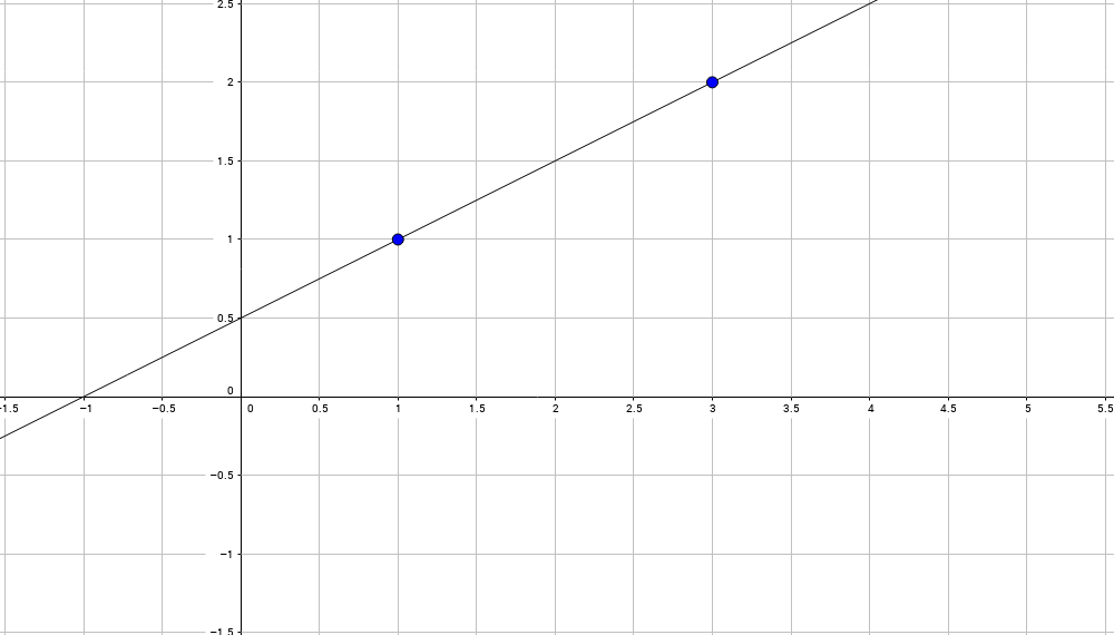
This line will have an equation like this one:

Alpha and beta are unknowns, but we do know two points on the line:

For convenience we can put in a matrix form:

A short excursus: what a matrix is? Matrix is nothing more than a 2D array of numbers. It is a way to store data, no more meaning attached. It depends on us how to interpret the data. From times to times I'll interpret it as a linear map, sometimes as a quadratic form, and even as a set of vectors, it should be clear from the context.
Let us replace actual matrices by their symbolic names:

Then we can easily find (alpha, beta):

To be more specific for our previous data:


And we obtain an equation of the straight line through (1,1) и (3,2):

Okay, it was really easy. What happens if we want to find a straight line through three points: (x0,y0), (x1,y1) и (x2,y2)?

Shucks. Three equations for two unknowns. A common mathematician would say that no solution exists (in general settings). But the programmer must have the job done. The boss won't listen for any excuses... He rewrites the previous system as follows:

And tries to find the solution that has minimum deviation from given specification. Let us call vector (x0,x1,x2) by i, vector (1,1,1) by j, and (y0,y1,y2) will be denoted as b:

In our case vectors i,j,b are three-dimensional, therefore, in general settings exact solution does not exits. Any vector (alpha* i + beta* j) lies in the plane generated by the basis (i, j). If b does not belong to the plane, no solution. What do we do? We are looking for a good trade-off. Let us denote by e(alpha, beta) our deviation from the exact equality:

Then we minimize this error:

Note that we do not minimize the norm of the vector e, but the square of the norm. Why? It is because both functions have the same minimum, but the squared norm is much nicer to minimize, because it is a smooth function in (alpha, beta) arguments, whereas the norm itself would give a conic function with no derivatives in the minimum. Ugly. The squared norm is convenient.
Obviously, the error is minimized when the vector e is orthogonal to the plane, generated by the basis i and j.

In other words, we are looking for a straight line minimizing the sum of squared distances (taken on a vertical lines) from the line itself to given points:

Let me abuse math for a second (very ill-formulated!): we take all possible straight lines through all pairs of points and the final line is the average between all of them:
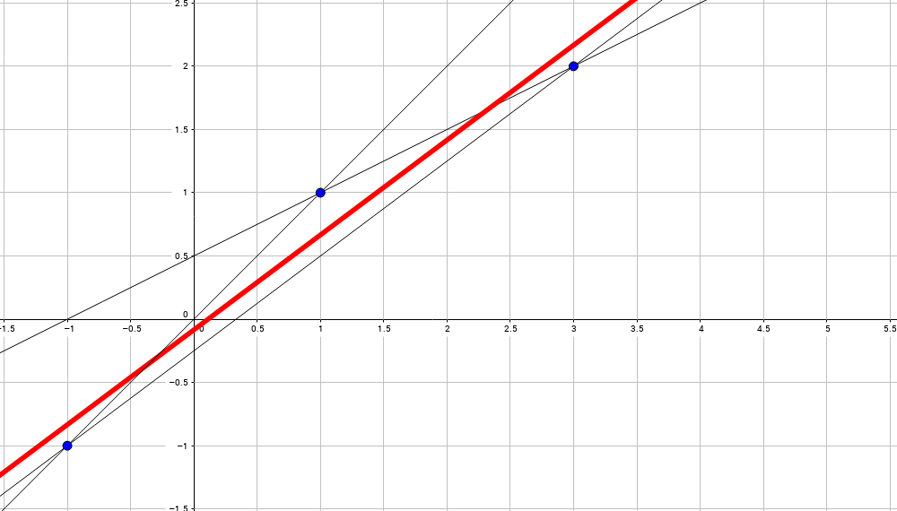
One more explication: we attach a (vertical) spring between all given points (three here) and the straight line. Then we are looking for the line in the equilibrium.
So, given a vector b and the feasible plane, generated by the column vectors of a matrix A (here (x0,x1,x2) and (1,1,1)), we are looking for a vector e with a minimum of its squared length. Obviously happens when e is orthogonal to the feasible plane:

We are looking for the vector x=(alpha, beta) such that:

So we solve this regular linear system for the vector x and we are done.
As a side note, it is easy to see that the vector x=(alpha, beta) minimizes the squared norm ||e(alpha, beta)||^2:

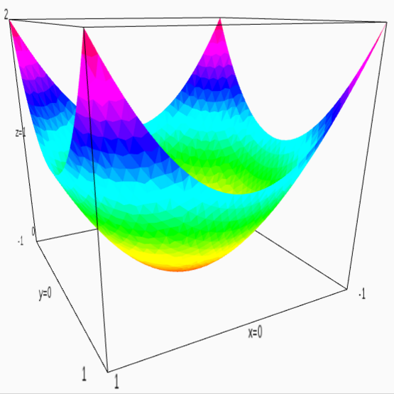
Now is a good moment to recall that a matrix can be interpreted as a quadratic form. For example, an identity matrix ((1,0),(0,1)) can be interpreted as the function x^2 + y^2:

All this acrobatics is known under the name of linear regression.
Usually least squares introductory lectures stop at the linear regression, but I need to get you a bit further. Let us consider a simple, but non-trivial problem. Let us say we have a triangulated surface that we need to smooth a bit. For example, here is a 3d model of my head:
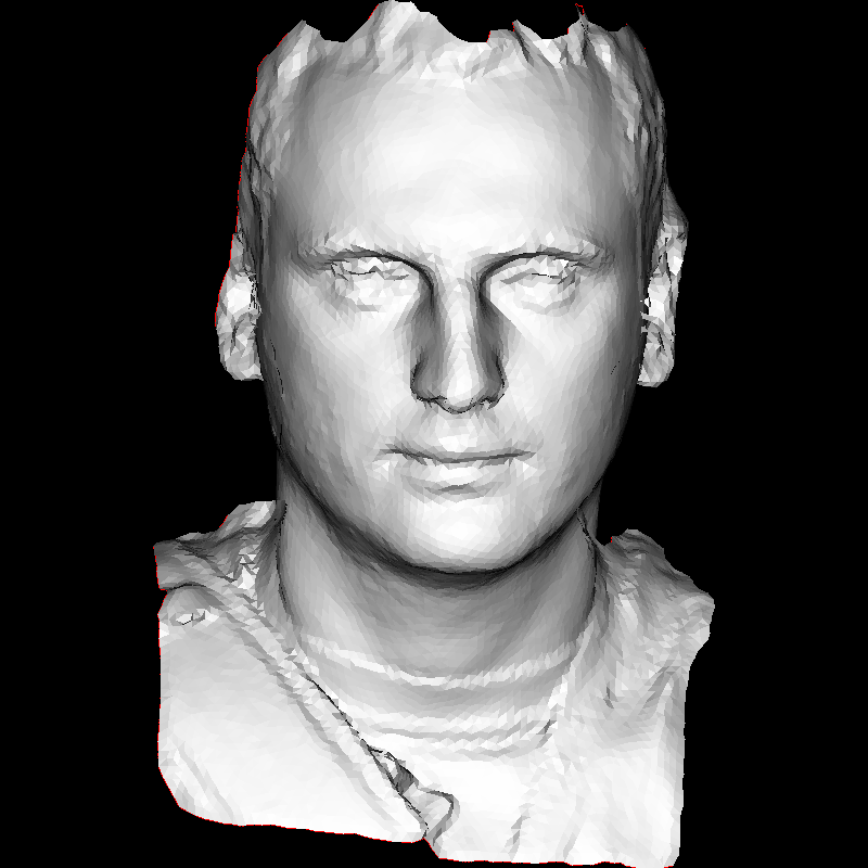
The starting code base is available here. In order to minimize external dependencies I took 3d model parser from my computer graphics course. I solve linear systems with OpenNL. It is a very nice solver easy to use and install: you simply put two files (.h and .c) in your project.
All the smoothing can be done with the following code:
    for (int d=0; d<3; d++) {
        nlNewContext();
        nlSolverParameteri(NL_NB_VARIABLES, verts.size());
        nlSolverParameteri(NL_LEAST_SQUARES, NL_TRUE);
        nlBegin(NL_SYSTEM);
        nlBegin(NL_MATRIX);

        for (int i=0; i<(int)verts.size(); i++) {
            nlBegin(NL_ROW);
            nlCoefficient(i, 1);
            nlRightHandSide(verts[i][d]);
            nlEnd(NL_ROW);
        }

        for (unsigned int i=0; i<faces.size(); i++) {
            std::vector<int> &face = faces[i];
            for (int j=0; j<3; j++) {
                nlBegin(NL_ROW);
                nlCoefficient(face[ j     ],  1);
                nlCoefficient(face[(j+1)%3], -1);
                nlEnd(NL_ROW);
            }
        }

        nlEnd(NL_MATRIX);
        nlEnd(NL_SYSTEM);
        nlSolve();

        for (int i=0; i<(int)verts.size(); i++) {
            verts[i][d] = nlGetVariable(i);
        }
    }
X, Y and Z coordinates are separable, I smooth it separately one from another. It means that I solve three different linear systems, and number of variables in these systems is equal to the number of vertices in the 3d model. First n rows of the matrix A have one 1 per row, and first n rows of the column-vector b contain corresponding vertex coordinates. It means that I put a spring between the new and the old vertex position: new positions should not be very far from the initial ones.
All following rows of the matrix A (faces.size()*3 = number of edges for all triangles in the mesh) have one 1 entry and one -1 entry per row, and corresponding entry of the vector b is zero. It means that I put a spring between all the vertices that share an edge.
Let us repeat once again: my variables are vertex positions, they can not go far from initial coordinates, but they do want to come near to their neighbours.
Here is the result:

It seems cool, the model is effectively smoothed, but it is shrunk and deviates from its initial border. Let us modify the source code a little bit:
        for (int i=0; i<(int)verts.size(); i++) {
            float scale = border[i] ? 1000 : 1;
            nlBegin(NL_ROW);
            nlCoefficient(i, scale);
            nlRightHandSide(scale*verts[i][d]);
            nlEnd(NL_ROW);
        }
For all vertices on the border instead of adding an equation v_i = verts[i][d] I add an equation 1000 * v_i = 1000 * verts[i][d]. What does it change? It changes the quadratic form of our error. A deviation from initial position on the border costs 1000*1000 times more than a deviation from initial position for other vertices. It means that we attached much more strong springs on the boundary vertices. The final solution prefers to stretch other springs. Here is the result:

Let us put two times stronger springs between neighbouring vertices:
                nlCoefficient(face[ j     ],  2);
                nlCoefficient(face[(j+1)%3], -2);
Naturally, the surface becomes smoother:

100 times stronger springs:

It shows an approximation for the so called minimal surface: imagine that we put a soap film on a wire loop. The soap will try to minimize its curvature while passing through the wire loop. Congratulations, you have just solved the famous Dirichlet problem. Sounds cool, but it simply means one linear system solved.
The source code can be found here.
Let us recall one more cool name. Imagine that we have this image:

The image is cool, but I do not like the chair.
I cut the image in two halves:


Create a mask by hand:

Then I put the following system of springs:
- the white part of the mask is attached to the left half of the image
- for all the left half I say that the difference between two neighboring pixels should be equal to the difference between corresponding pixels in the right half
    for (int i=0; i<w*h; i++) {
        if (m.get(i%w, i/w)[0]<128) continue;
        nlBegin(NL_ROW);
        nlCoefficient(i, 1);
        nlRightHandSide(a.get(i%w, i/w)[0]);
        nlScaleRow(100);
        nlEnd(NL_ROW);
    }

    for (int i=0; i<w-1; i++) {
        for (int j=0; j<h-1; j++) {
            for (int d=0; d<2; d++) {
                nlBegin(NL_ROW);
                int v1 = b.get(i,   j    )[0];
                int v2 = b.get(i+d, j+1-d)[0];
                nlCoefficient( i   + j     *w,  1);
                nlCoefficient((i+d)+(j+1-d)*w, -1);
                nlRightHandSide(v1-v2);
                nlScaleRow(10);
                nlEnd(NL_ROW);
            }
        }
    }
Here is the result:

The source code and the images can be found here
As I simply wanted to show you how it is possible to use least squares, the above example is quick and dirty, it is a tutorial code. Let me show you a real life example.
I have plenty of photos of printed fabrics like this one:

The goal is to create seamless textures from this kind of photos. First of all I am looking for a repeating pattern (automatically, by means of phase correlation):

If I cut out this quad, then because of non-rigid fabric and lens distortions I will obtain clearly visible seams. Here is the quad mapped on a rectangle, repeated 4 times:

Here is a zoom that shows the seam:

So I won't cut along a straight line, the cut is curved (I used graph-cut technique):

Here is the pattern repeated four times:

And a zoom on a fragment:

It is much better than before, the cut follows the pattern, but we still see the seam because of the uneven lighting. Here is the good moment to use our least-squares solver for the Poisson problem. Here is the final result (clickable):

We obtained a perfectly seamless texture from a so-so photo. Do not be afraid of math and you will have your engineering happiness!