Least squares view on the linear quadratic regulator
My original post in Russian is available here.
— Hi, my name is %username and I secretly disclose the brackets in sums expressed in sigma notation to understand what is happening.
— Hi %username!
I have few students who want to implement a segway-style two-wheeled balancing robot like this one (clickable, video underneath):

They thought to use a PID regulator, but failed to find good coefficients and came to ask for a help. I am not an expert in the control theory, however I saw a guy to mention that he failed with PID, but that LQR worked out for him. So I took my time to document me on the LQR, and I wanted to explain to you whait I learned. It is also a good opportunity to show you how I read math text, it is a major part of my work. This page does NOT explain how to build balancing bots, it is an introduction to LQR. I suppose that you have a basic understanding of least squares, for example, read this page.
Well, whenever I see something new for me, I check wikipedia. In this particular article all I can see is an awful wall of text that I can not understand. However one sentence catches my eye:
The theory of optimal control is concerned with operating a dynamic system at minimum cost. The case where the system dynamics are described by a set of linear differential equations and the cost is described by a quadratic function is called the LQ problem.
This sentence means that for a physical object (e.g. a car) the control (e.g. steering wheel angle) can be chosen by minimizing some cost function. Cool, I can sense least squares problem and this is good.
Okay, let us contunue reading:
Finite-horizon, continuous-time LQR, [scary formulas]
Skipping, I do not want to understand these. Computing continuous functions by hand can be really messy.
Infinite-horizon, continuous-time LQR, [even more scary formulas]
Mein gott, improper integrals. Skipping, let us check if there is something interesting below...
Finite-horizon, discrete-time LQR
Cool, I like discrete systems. There is a system that can be described by a set of values x, we observe it every few moments (any time interval for me equals one second unless specified otherwise). No more derivatives, they can be approximated as (x_{k+1}-x_{k})/1 sec = x_{k+1}-x_{k}. All we have to do now is to understand what x_k is.
Let us perform an imaginary experiment. In his book Feynman wrote how he read all the equations:
Actually, there was a certain amount of genuine quality to my guesses. I had a scheme, which I still use today when somebody is explaining something that I'm trying to understand: I keep making up examples. For instance, the mathematicians would come in with a terrific theorem, and they're all excited. As they're telling me the conditions of the theorem, I construct something which fits all the conditions. You know, you have a set (one ball) — disjoint (two balls). Then the balls turn colors, grow hairs, or whatever, in my head as they put more conditions on. Finally they state the theorem, which is some dumb thing about the ball which isn't true for my hairy green ball thing, so I say, "False!"
Even Feynman instantiated all the formulas, so I humbly follow his approach. Let us say we have a car with some initial speed. The goal is to hit the gas pedal, thus influencing the acceleration, to reach some given final speed.
So, let us suppose that we have an ideal car with the following law:

x_k - is the speed of the car at the second k, u_k - is the position of the gas pedal at the same moment, we can interpret it as an acceleration. So, we are starting with some speed x_0, and then we perform a numerical integration. Scary words aside, if we have a speed x_0 and acceleration u_0, then in one second the speed will be equal to x_0 + u_0. Please note that the units are correct: I am not summing m/s with (m/s)/s, the speed increment will be obtained by multiplying the acceleration by 1 second time interval. All coefficients in my imaginary experiments are equal either to 0 or 1.
So to understand what is happening I write the following code. I write tons of disposable code that I throw away immediately. As usual, I use OpenNL to solve sparse linear systems of equations.
#include <iostream>
#include "OpenNL_psm.h"

int main() {
    const int N = 60;
    const double xN = 2.3;
    const double x0 = .5;
    const double hard_penalty = 100.;

    nlNewContext();
    nlSolverParameteri(NL_NB_VARIABLES, N*2);
    nlSolverParameteri(NL_LEAST_SQUARES, NL_TRUE);
    nlBegin(NL_SYSTEM);
    nlBegin(NL_MATRIX);

    nlBegin(NL_ROW); // x0 = x0
    nlCoefficient(0, 1);
    nlRightHandSide(x0);
    nlScaleRow(hard_penalty);
    nlEnd(NL_ROW);

    nlBegin(NL_ROW); // xN = xN
    nlCoefficient((N-1)*2, 1);
    nlRightHandSide(xN);
    nlScaleRow(hard_penalty);
    nlEnd(NL_ROW);

    nlBegin(NL_ROW); // uN = 0, for convenience, normally uN is not defined
    nlCoefficient((N-1)*2+1, 1);
    nlScaleRow(hard_penalty);
    nlEnd(NL_ROW);

    for (int i=0; i<N-1; i++) {
        nlBegin(NL_ROW); // x{i+1} = xi + ui
        nlCoefficient((i+1)*2  , -1);
        nlCoefficient((i  )*2  ,  1);
        nlCoefficient((i  )*2+1,  1);
        nlScaleRow(hard_penalty);
        nlEnd(NL_ROW);
    }

    for (int i=0; i<N; i++) {
        nlBegin(NL_ROW); // xi = xN, soft
        nlCoefficient(i*2, 1);
        nlRightHandSide(xN);
        nlEnd(NL_ROW);
    }

    nlEnd(NL_MATRIX);
    nlEnd(NL_SYSTEM);
    nlSolve();

    for (int i=0; i<N; i++) {
        std::cout << nlGetVariable(i*2) << " " <<  nlGetVariable(i*2+1) << std::endl;
    }

    nlDeleteContext(nlGetCurrent());
    return 0;
}
Let us find what is happening in the source code. First of all I say that N=60, i give 60 seconds for the car to accelerate. Then I say that the goal speed is 2.3 m/s, the initial speed is .5 m/s (I took arbitrary values). I will have 60*2 variables: 60 speed values as well 60 acceleration values (strictly speaking, there are 59 accelerations, but it is easier for me to say we have 60 and force the last to be zero)
Therefore, I have 2*N variables (N=6), even variables (as every programmer I start counting from zero) are for the speed, odd variables are for the acceleration. I specify the initial and the final speed by these lines of code, they say that the initial speed must be equal to x0 (.5m/s), the final speed equal to xN (2.3m/s):
    nlBegin(NL_ROW); // x0 = x0
    nlCoefficient(0, 1);
    nlRightHandSide(x0);
    nlScaleRow(hard_penalty);
    nlEnd(NL_ROW);

    nlBegin(NL_ROW); // xN = xN
    nlCoefficient((N-1)*2, 1);
    nlRightHandSide(xN);
    nlScaleRow(hard_penalty);
    nlEnd(NL_ROW);
We know that the car must obey x{i+1} = xi + ui, so let us add N-1 equations in our system:
    for (int i=0; i<N-1; i++) {
        nlBegin(NL_ROW); // x{i+1} = xi + ui
        nlCoefficient((i+1)*2  , -1);
        nlCoefficient((i  )*2  ,  1);
        nlCoefficient((i  )*2+1,  1);
        nlScaleRow(hard_penalty);
        nlEnd(NL_ROW);
    }
So, we have added all the hard constraints in our system. But what are we looking to optimize for? For the first run let us say that we want x_i to reach the final speed xN as fast as it can:
    for (int i=0; i<N; i++) {
        nlBegin(NL_ROW); // xi = xN, soft
        nlCoefficient(i*2, 1);
        nlRightHandSide(xN);
        nlEnd(NL_ROW);
    }
Our system is ready, we specified hard constraints for the behaviour of the dynamics, as well as the quadratic cost for the solution quality. Let us run the code and see what we obtain for the solution x_i, u_i. Here the red line is the speed, the green one is the acceleration:
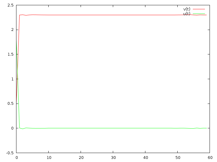
Oookaay, the car indeed accelerates to the given speed, but the acceleration is waaay to high for a real physical system. Let us modify our cost function and say that the acceleration is to be as low as possible:
    for (int i=0; i<N; i++) {
        nlBegin(NL_ROW); // ui = 0, soft
        nlCoefficient(i*2+1, 1);
        nlEnd(NL_ROW);
    }
Here is the corresponding commit, and the solution looks as follows:
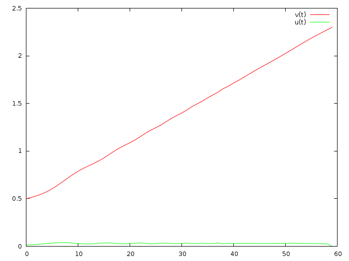
That is better for a physical system, but one minute to accelerate from .5m/s to 2.3m/s? Come on! Let us add both wishes to attain the final speed as fast as possible, but to keep overall acceleration as low as we can:
    for (int i=0; i<N; i++) {
        nlBegin(NL_ROW); // ui = 0, soft
        nlCoefficient(i*2+1, 1);
        nlEnd(NL_ROW);

        nlBegin(NL_ROW); // xi = xN, soft
        nlCoefficient(i*2, 1);
        nlRightHandSide(xN);
        nlEnd(NL_ROW);
    }
Here is the corresponding commit, and the solution is:
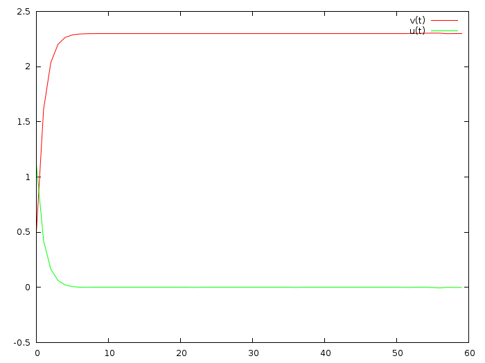
This graph is reasonable, we attain the goal in few seconds and the acceleration is bearable. Therefore can conclude that quick convergence to the goal and limitation of the control are concurrent goals.
Note that we are at the first sentence of the "Finite-horizon, discrete-time LQR" wiki paragraph. All the rest is filled with ugly formulas that I do not understand. Quite often you need to surf through the text to grasp the keywords you know to project the text onto the basis of your personal knowledge.
So let us sum up: starting from the initial + final settings + number of seconds in between we can find ideal control curve u_k to apply. That is cool, but how can we apply this to our segway problem? Should we resolve all this big system at each time step? I do not know, let us continue reading the wiki article:
with a performance index defined as

the optimal control sequence minimizing the performance index is given by
where [AARGH WHAT IS THAT?!]
Well, let us stop a moment. I do not really understand what goes after "J=...", but it looks like a quadratic function that we have just tried: reach goal quickly with little efforts.
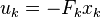
But then I see the magic formula u_k = -F x_k. Stop. This looks really, really interesting. If we recall our 1D example, it means that the gas pedal position (green curve) must be equal to the speed (red curve), multiplied by a constant. If we look at the above graph, it does look so!
Let us try to derive the equations for our 1D example. So we have the quality of control function J:
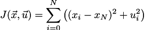
We want to minimize it under the constraints of the system dynamics:
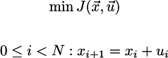
Wait-wait-wait, do you see x_k^T Q x_k expression in the wiki? In our case it would be simple x_k^2, but our equation has (x_k-x-N)^2 term. Gosh. The authors suppose that the final goal is the zero vector! Why on EARTH isn't it mentioned?!
After realizing this I take a deep breath and continue. Now let us express all x_k through u_k in the J function in order to eliminate constraints/redundant variables.
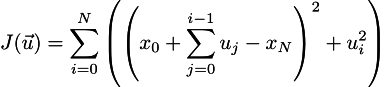
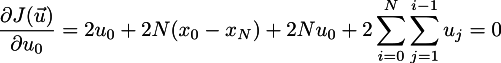
Cool, now it is the time for the brackets disclosure (cf. the epigraph):
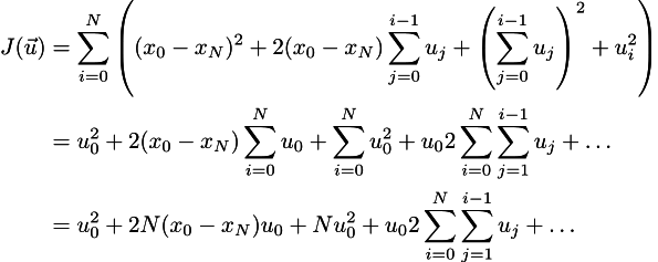
The dots mean all the stuff that does not depend on the u_0. We are looking for the minimum, so the partial derivative w.r.t. to u_0 must be zero:
Finally, we obtain that the control u_0 is optimal only if it has the following expression:
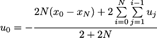
Please note that this expression contains other unknowns u_i, but there is one point: I do not want my car to accelerate all the minute, I gave the minute simply as a largely sufficient time, nothing forbids to provide one hour. Roughly speaking, the member depending on u_i is all the (bounded) work on the acceleration, it does not depend on N. If N is sufficiently large, then optimal u_0 depends linearly only on the difference between x_0 and x_N!
Therefore, the control loop is really simple: we model the system, compute the magical coefficent F that links u_k and x_k : u_k = -F (x_k - x_N) and implement in the final controller a simple proportional regulator!
To be completely honest, up to this point I did not write the code, all the above can be done with napkin draft. Here is the first code I actually wrote for the problem, let me list it here:
#include <iostream>
#include <vector>
#include "OpenNL_psm.h"

int main() {
    const int N = 60;
    const double x0 = 3.1;
    const double v0 = .5;
    const double hard_penalty = 100.;
    const double rho = 16.;

    nlNewContext();
    nlSolverParameteri(NL_NB_VARIABLES, N*3);
    nlSolverParameteri(NL_LEAST_SQUARES, NL_TRUE);
    nlBegin(NL_SYSTEM);
    nlBegin(NL_MATRIX);

    nlBegin(NL_ROW);
    nlCoefficient(0, 1); // x0 = 3.1
    nlRightHandSide(x0);
    nlScaleRow(hard_penalty);
    nlEnd(NL_ROW);

    nlBegin(NL_ROW);
    nlCoefficient(1, 1); // v0 = .5
    nlRightHandSide(v0);
    nlScaleRow(hard_penalty);
    nlEnd(NL_ROW);

    nlBegin(NL_ROW);
    nlCoefficient((N-1)*3, 1); // xN = 0
    nlScaleRow(hard_penalty);
    nlEnd(NL_ROW);

    nlBegin(NL_ROW);
    nlCoefficient((N-1)*3+1, 1); // vN = 0
    nlScaleRow(hard_penalty);
    nlEnd(NL_ROW);

    nlBegin(NL_ROW); // uN = 0, for convenience, normally uN is not defined
    nlCoefficient((N-1)*3+2, 1);
    nlScaleRow(hard_penalty);
    nlEnd(NL_ROW);

    for (int i=0; i<N-1; i++) {
        nlBegin(NL_ROW); // x{N+1} = xN + vN
        nlCoefficient((i+1)*3  , -1);
        nlCoefficient((i  )*3  ,  1);
        nlCoefficient((i  )*3+1,  1);
        nlScaleRow(hard_penalty);
        nlEnd(NL_ROW);

        nlBegin(NL_ROW); // v{N+1} = vN + uN
        nlCoefficient((i+1)*3+1, -1);
        nlCoefficient((i  )*3+1,  1);
        nlCoefficient((i  )*3+2,  1);
        nlScaleRow(hard_penalty);
        nlEnd(NL_ROW);
    }

    for (int i=0; i<N; i++) {
        nlBegin(NL_ROW); // xi = 0, soft
        nlCoefficient(i*3, 1);
        nlEnd(NL_ROW);

        nlBegin(NL_ROW); // vi = 0, soft
        nlCoefficient(i*3+1, 1);
        nlEnd(NL_ROW);

        nlBegin(NL_ROW); // ui = 0, soft
        nlCoefficient(i*3+2, 1);
        nlScaleRow(rho);
        nlEnd(NL_ROW);
    }

    nlEnd(NL_MATRIX);
    nlEnd(NL_SYSTEM);
    nlSolve();

    std::vector<double> solution;
    for (int i=0; i<3*N; i++) {
        solution.push_back(nlGetVariable(i));
    }

    nlDeleteContext(nlGetCurrent());

    for (int i=0; i<N; i++) {
        for (int j=0; j<3; j++) {
            std::cout << solution[i*3+j] << " ";
        }
        std::cout << std::endl;
    }

    return 0;
}
Here the problem is the same as before, but we have two variables in the system: car's coordinate and its speed. Starting from given position and speed (x0, v0), we need to reach final position and speed (0,0). In other words, we need to stop the car in the origin of our coordinate system. The dynamics of our system can be described with two equations x_{k+1} = x_k + v_k, and v_{k+1} = v_k + u_k.
Since this code looks exactly the same as the previous one, it should not pose any problems. Here is the solution:
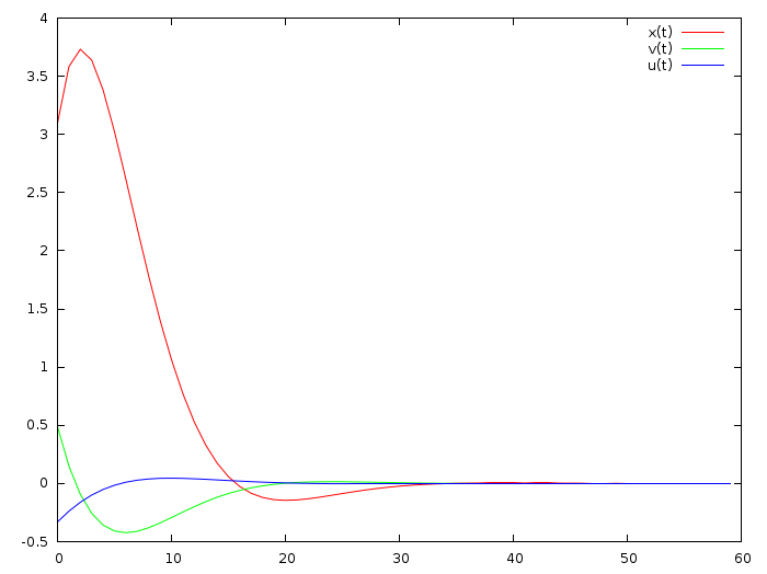
Red curve - coordinate, green one - speed, blue one - gas pedal state. If the wiki is right, the blue curve must be a weighted sum of the red and green curves. Hmm, is that so? Let us find out!
So we need to find two numbers a and b such that u_i = ax_i + bv_i. And this is nothing else than simple linear regression. Let us run the following program. This program computes all three curves as before, and then computes for the values a and b such that blue curve = ared curve + bgreen curve.
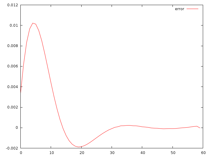
Here is the difference between actual u_i and the weighted sum of red and green curves:
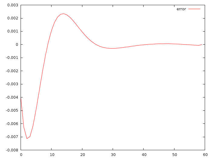
The maximum deviation between u_i and the weighted difference is less than (1cm/s)/s, cool! The above commit gives the values a=-0.0513868, b=-0.347324. The deviation is small, but we started from the same initial position. What happens if we change it? Would we predict the optimal control as well? Let us find out.
I drastically changed initial settings, but kept magical values a and b from the previous computation.
Here is the deviation between the optimal control and very dumb prediction obtained with the following procedure:
    double xi = x0;
    double vi = v0;
    for (int i=0; i<N; i++) {
        double ui = xi*a + vi*b;
        xi = xi + vi;
        vi = vi + ui;
        std::cout << (ui-solution[i*3+2]) << std::endl;
    }
No Riccati differential equations proposed by the wiki!
The above car problem can be solved with few lines of Matlab code:
A=[1 1;0 1];
B=[0;1];
Q=eye(2);
R=256;
F=-dlqr(A,B,Q,R)
It gives us the solution F=-[0.052 0.354] that is very close to our guess F=-[0.051, 0.347]!
To create an LQR controller, there are two main difficulties:
a) find good transition (kinematic) matrices A and B that depend on masses, moments of inertia and stuff b) find a good balance between concurrent goals: reach the goal quickly, but do not go over maximum control possibility
LQR is a great method of control for a linearized system. The only problem that it asks for a complete knowledge of the system state, it is not always doable. For example, we can only guess the angle of the segway from accelerometer and gyroscope readings. But it is a story for another article.
I wanted to reach three goals: a) understand what LQR is b) explain it to my students and you c) show you that I (as well as most of people I know) understand very little in math papers, it is sad, but not at all a catastrophic situation. Try to find things you know and to project all the things you do not know onto your proper basis of knowledge.
I hope that I succeeded in these three points. I am not a specialist in the control theory, if you have any corrections please do let me know.
Enjoy!