This repository enables the public to investigate stock movement prediction backtesting result generated using Stockenja's Crystal Ball technology. You can find the backtesting data and script to analyze the data in this repo.
At Stockenja, we believe that there are right timings to invest in different stocks and those timings can be predicted with fair amount of accuracy. This project was created to prove this hypothesis.
Furthermore, we have received many questions about Crystal Ball's accuracy/success rate. While we would like to be able to display the past success rate for each ticker on our site, the cost associated with it is just not possible at this current moment. In order to compute the success rate for one ticker with a period of 2 years timeframe, it will take us 5 minutes to do so. This will not be a good user experience and requires a lot of computational resources.
Therefore, we chose to publish some benchmark data that contains Crystal Ball's computed probability and a simple script to allow everyone to play with the data to explore the validity of our prediction algorithm.
To keep it simple, we want to prove that it is possible to predict stock movement using Crystal Ball's computed probability.
To confirm that Crystal Ball's probability is legit, we apply our algorithm in some time in the past Tp and get an associated probability for N trading days later. To obtain meaningful result, our prediction algorithm does not have any information beyond Tp during simulation/experiment.
To generate the data required to analyze the validity of our probability, we followed the steps below:
-
We picked 4 different securities, namely: SPY, AMZN, GLD and XBI. SPY is the SP500 index fund, which has the lowest volatility among all the selected securities. AMZN (Amazon) and XBI (US Biotech Sector Index Fund) are highly volatile securities but still has a strong upwards trend. Finally, there is GLD (Gold ETF). GLD is very special and actually behaves relatively unexpectedly. Prior to 2012, GLD has a strong upward trend but it went stagnant after that. While it is not very volatile, its trend is hard to predict.
We chose different securities because we wanted to make sure our probabilities is representative for all securities.
-
Next, we selected some of the simulation parameters to be the following:
- The total number of trading days to simulate is 504 trading days(i.e. 2 years)
- The number of days to predict ahead is 20 trading days (i.e. 1 month)
- The last date of simulation is 2018-01-01. Therefore, our first date of simulation is 2016-01-01.
-
With these parameters set, the next step is to simulate and compute the probabilities plus the actual 20 days return for each trading day Tp. We start by extracting all the price data and computing the technical indicators required. We start with the last date, which is 2018-01-01. The reason for starting with the last date first is to avoid getting the large amount of price data from the database for every single timestep.
Once the probability of Tp is computed, we save it to a list and remove all the price data and indicators associated with Tp. (This ensure our prediction algorithm does not contain any future data, which simulate the fact that the algorithm is living in the past). Then, we set
Tp = Tp -1.This simulation stops when
Tp = 2016-01-01. -
Once the simulation stops, we store the useful output into a JSON file and include it into this project for analysis purposes.
-
We run the file "analyze-data.py" to compute the success rate or accuracy of our prediction algorithm. We will issue a buy signal when the probability on Tp is greater than the threshold, Pt. Conversely, we issue a short (sell) signal when the probability of Tp is smaller than 1-Pt. We consider a buy signal to be successful when the 20 days return is greater than 0 and vice versa.
Using the above simulation setup, we ran the script "analyze-data.py" for different probability threshold. You can think about the probability threshold as a buy signal. When the probability is above some threshold, then we will buy a security/stock. We will look at the 20 days later return and decide if we have successfully predicted stock movement (which is basically if it larger than 0% return or smaller).
When we set the probability threshold to 70%, we get an average of 81% successful prediction rate. The total number of prediction made is around 500 times for all 4 securities. The actual success rate for each of the 4 securities is shown in the figure below:
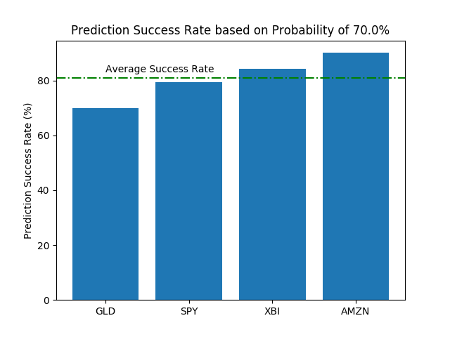
The fact that we get 81% success rate when we set a threshold of 70% implies that our algorithm is doing its job. Of course, one could argue that this success rate is attributed to the bull market. We would not argue against this statement and we do believe that 81% success rate seems a bit high. But, it is worth noting that GLD has a success rate at 70% too. Gold did not rally strongly in the period of year 2016-2018. Based on these results, we believe that we are on the right track to creating a revolutionary prediction algorithm.
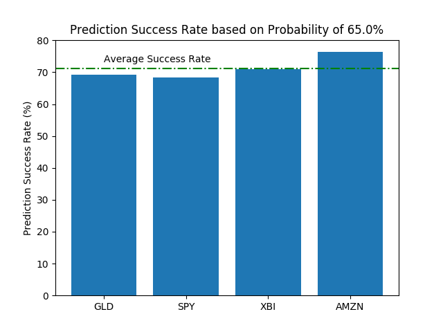
Let's take a look at the results when the probability threshold is at 65%. We expect the successful prediction rate to drop. Running the script, we get an overall successful prediction rate of 71%. The total number of predictions made is roughly 1000 times. The actual success rate for each of the 4 securities is shown in the figure below:
Finally, let's take a look at the results when the probability threshold is at 80%. We expect the successful prediction rate to be higher than the one obtained by 70% (which is 81%). Running the script, we get an overall successful prediction rate of 86%. The total number of predictions made is roughly 110 times. The actual success rate for each of the 4 securities is shown in the figure below:
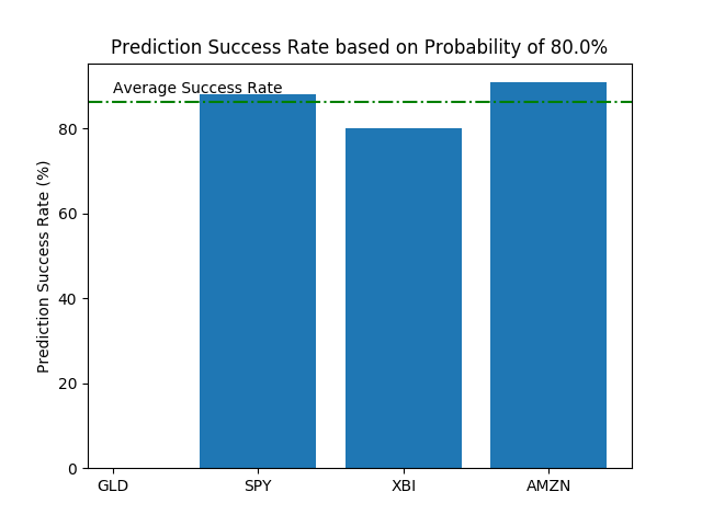
In the figure above, it seems like GLD prediction rate is 0%. But, that is not the case. Since 80% threshold is too high, the script cannot find any probability that is larger than 80%. Therefore, it is actually not issuing any buy signal. You can see that no predictions were made for GLD if you run the script.
Based on the above results, we are quite confident that using probabilities is right approach to predicting stock movements. Of course, more research is needed to validate that if Crystal Ball will yield similar results for different time frames. Our hypothesis is that it will yield successful results because our technology is based on mathematical fundamentals, which is probability.
To start, create virtual environment:
virtualenv --python=python3.6 backtest-result-env
Next, we want to install the dependencies:
pip install -r requirements.txt
To enable plotting in your shell, please install the following package:
sudo apt-get install python-tk python3-tk tk-dev
Done.
Simply change directory to the cloned repo and run:
python analyze-data.py
If you have any questions or would like to seek for collaboration, please feel free to send us an email at hello@stockenja.com.
This repo is licensed under the MIT license.