Package for making elements of technical analysis of a stock easier. This package is meant to be a starting point for you to develop your own. As such, all the instructions for installing/setup will be assuming you will continue to develop on your end.
This section will show some of the functionality of each class; however, it is by no means exhaustive.
from stock_analysis import StockReader

reader = StockReader("2017-01-01", "2018-12-31")

# get bitcoin data in USD
bitcoin = reader.get_bitcoin_data("USD")

# get faang data
fb, aapl, amzn, nflx, goog = (
    reader.get_ticker_data(ticker) for ticker in ["FB", "AAPL", "AMZN", "NFLX", "GOOG"]
)

# get S&P 500 data
sp = reader.get_index_data("S&P 500")from stock_analysis import group_stocks, describe_group
faang = group_stocks(
{"Facebook": fb, "Apple": aapl, "Amazon": amzn, "Netflix": nflx, "Google": goog}
)
# describe the group
describe_group(faang)Groups assets by date and sums columns to build a portfolio.
from stock_analysis import make_portfolio

faang_portfolio = make_portfolio(faang)Be sure to check out the other methods here for different plot types, reference lines, shaded regions, and more!
Evolution over time:
import matplotlib.pyplot as plt
from stock_analysis import StockVisualizer

netflix_viz = StockVisualizer(nflx)

ax = netflix_viz.evolution_over_time(
    "close", figsize=(10, 4), legend=False, title="Netflix closing price over time"
)
netflix_viz.add_reference_line(
    ax,
    x=nflx.high.idxmax(),
    color="k",
    linestyle=":",
    label=f"highest value ({nflx.high.idxmax():%b %d})",
    alpha=0.5,
)
ax.set_ylabel("price ($)")
plt.show()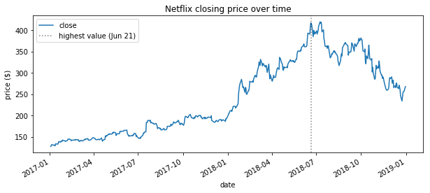
After hours trades:
netflix_viz.after_hours_trades()
plt.show()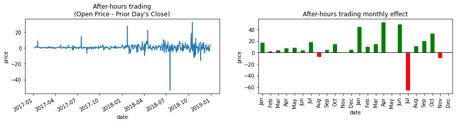
Differential in closing price versus another asset:
netflix_viz.fill_between_other(fb)
plt.show()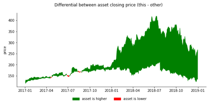
Candlestick plots with resampling (uses mplfinance):
netflix_viz.candlestick(
    resample="2W", volume=True, xrotation=90, datetime_format="%Y-%b -"
)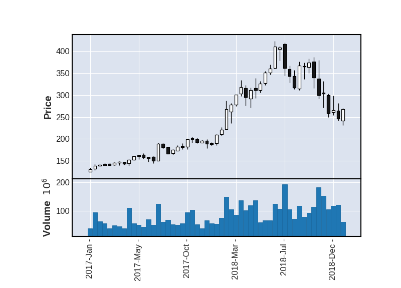
Note: run help() on StockVisualizer for more visualizations
Correlation heatmap:
from stock_analysis import AssetGroupVisualizer

faang_viz = AssetGroupVisualizer(faang)
faang_viz.heatmap(True)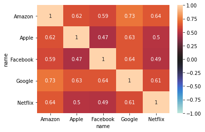
Note: run help() on AssetGroupVisualizer for more visualizations. This object has many of the visualizations of the StockVisualizer class.
Below are a few of the metrics you can calculate.
from stock_analysis import StockAnalyzer

nflx_analyzer = stock_analysis.StockAnalyzer(nflx)
nflx_analyzer.annualized_volatility()Methods of the StockAnalyzer class can be accessed by name with the AssetGroupAnalyzer class's analyze() method.
from stock_analysis import AssetGroupAnalyzer

faang_analyzer = AssetGroupAnalyzer(faang)
faang_analyzer.analyze("annualized_volatility")

faang_analyzer.analyze("beta")from stock_analysis import StockModelerdecomposition = StockModeler.decompose(nflx, 20)
fig = decomposition.plot()
plt.show()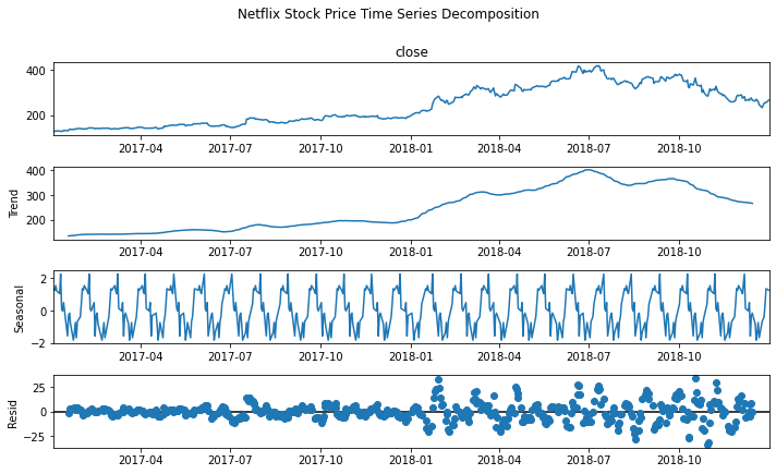
Build the model:
arima_model = StockModeler.arima(nflx, 10, 1, 5)Check the residuals:
StockModeler.plot_residuals(arima_model)
plt.show()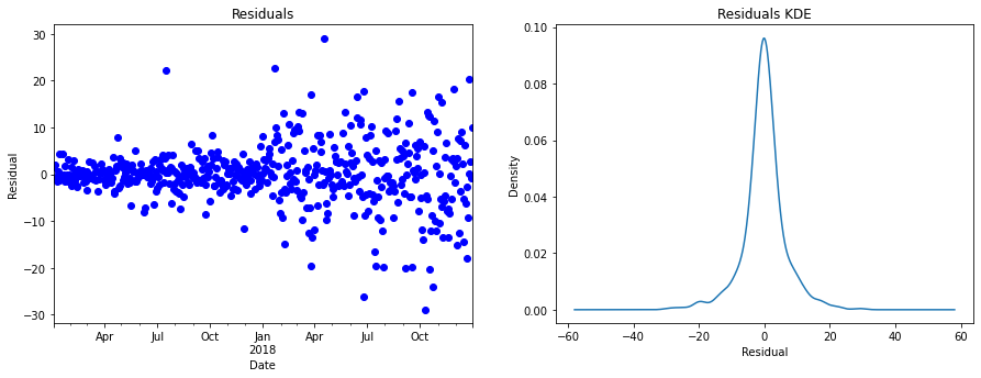
Plot the predictions:
arima_ax = StockModeler.arima_predictions(
    arima_model, start=start, end=end, df=nflx, ax=axes[0], title="ARIMA"
)
plt.show()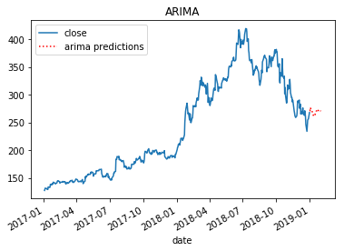
Build the model:
X, Y, lm = StockModeler.regression(nflx)Check the residuals:
StockModeler.plot_residuals(lm)
plt.show()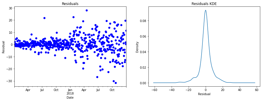
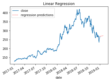
Plot the predictions:
linear_reg = StockModeler.regression_predictions(
    lm, start=start, end=end, df=nflx, ax=axes[1], title="Linear Regression"
)
plt.show()