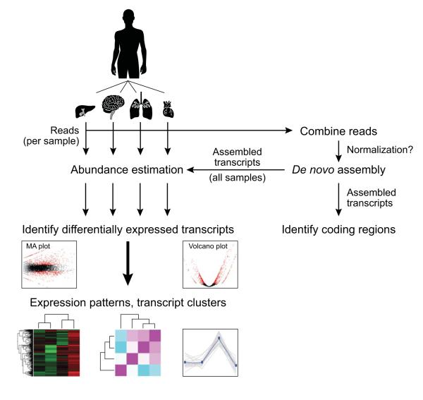
Trinity De novo Transcriptome Assembly Workshop
The following details the steps involved in:
- Generating a Trinity de novo RNA-Seq assembly
-
Inspecting the assembly in the context of a reference genome (when one is available)-
Mapping reads and Trinity transcripts to a target genome sequence (when one is available). -
Visualizing the aligned reads and transcripts in comparison to reference transcript annotations.
-
- Identifying differentially expressed transcripts using EdgeR and various Trinity-included helper utilities.
All required software and data are provided pre-installed on a VirtualBox image. Be sure to run the workshop VM and open a terminal.
After installing the VM, be sure to quickly update the contents of the rnaseq_workshop_data directory by:
    %   cd RNASeq_Trinity_Tuxedo_Workshop

    %   git pull
This way, you’ll have the latest content, including any recent bugfixes.
This demo uses RNA-Seq data corresponding to Schizosaccharomyces pombe (fission yeast), involving paired-end 76 base strand-specific RNA-Seq reads corresponding to four samples: Sp_log (logarithmic growth), Sp_plat (plateau phase), Sp_hs (heat shock), and Sp_ds (diauxic shift).
There are 'left.fq' and 'right.fq' FASTQ formatted Illlumina read files for each of the four samples. All RNA-Seq data sets can be found in the RNASEQ_data/ subdirectory.
Also included is a 'genome.fa' file corresponding to a genome sequence, and annotations for reference genes ('genes.bed' or 'genes.gff3'). These resources can be found in the GENOME_data/ subdirectory.
Note, although the genes, annotations, and reads represent genuine sequence data, they were artificially selected and organized for use in this tutorial, so as to provide varied levels of expression in a very small data set, which could be processed and analyzed within an approximately one hour time session and with minimal computing resources.
The commands to be executed are indicated below after a command prompt '%'. You can type these commands into the terminal, or you can simply copy/paste these commands into the terminal to execute the operations.
To avoid having to copy/paste the numerous commands shown below into a unix terminal, the VM includes a script ‘runTrinityDemo.pl’ that enables you to run each of the steps interactively. To begin, simply run:
% ./runTrinityDemo.pl
Note, by default and for convenience, the demo will show you the commands that are to be executed. This way, you don’t need to type them in yourself.
The protocol followed is that described here: http://www.ncbi.nlm.nih.gov/pmc/articles/PMC3875132/
Below, we refer to ${TRINITY_HOME}/ as the directory where the Trinity software is installed, and '%' as the command prompt.
To generate a reference assembly that we can later use for analyzing differential expression, we'll combine the read data sets for the different conditions together into a single target for Trinity assembly. We do this by providing Trinity with a list of all the left and right fastq files to the --left and --right parameters as comma-delimited like so:
   %   ${TRINITY_HOME}/Trinity --seqType fq --SS_lib_type RF  \
           --left RNASEQ_data/Sp_log.left.fq.gz,RNASEQ_data/Sp_hs.left.fq.gz,RNASEQ_data/Sp_ds.left.fq.gz,RNASEQ_data/Sp_plat.left.fq.gz \
           --right RNASEQ_data/Sp_log.right.fq.gz,RNASEQ_data/Sp_hs.right.fq.gz,RNASEQ_data/Sp_ds.right.fq.gz,RNASEQ_data/Sp_plat.right.fq.gz \
           --CPU 2 --max_memory 1G
Running Trinity on this data set may take 10 to 15 minutes. You’ll see it progress through the various stages, starting with Jellyfish to generate the k-mer catalog, then followed by Inchworm, Chrysalis, and finally Butterfly. Running a typical Trinity job requires ~1 hour and ~1G RAM per ~1 million PE reads. You'd normally run it on a high-memory machine and let it churn for hours or days.
The assembled transcripts will be found at ‘trinity_out_dir/Trinity.fasta’.
Just to look at the top few lines of the assembled transcript fasta file, you can run:
% head trinity_out_dir/Trinity.fasta
and you can see the Fasta-formatted Trinity output:
>TRINITY_DN0_c0_g1_i1 len=1894 path=[1872:0-1893] [-1, 1872, -2]
GTATACTGAGGTTTATTGCCTGTAACGGGCAAACTCGAGCAGTTCAATCACGAGGAGATT
ACCAGAAAACACTCGCTATTGCTTTGAAAAAGTTTAGCCTTGAAGATGCTTCAAAATTCA
TTGTATGCGTTTCACAGAGTAGTCGAATTAAGCTGATTACTGAAGAAGAATTTAAACAAA
TTTGTTTTAATTCATCTTCACCGGAACGCGACAGGTTAATTATTGTGCCAAAAGAAAAGC
CTTGTCCATCGTTTGAAGACCTCCGCCGTTCTTGGGAGATTGAATTGGCTCAACCGGCAG
CATTATCATCACAGTCCTCCCTTTCTCCTAAACTTTCCTCTGTTCTTCCCACGAGCACTC
AGAAACGAAGTGTCCGCTCAAATAATGCGAAACCATTTGAATCCTACCAGCGACCTCCTA
GCGAGCTTATTAATTCTAGAATTTCCGATTTTTTCCCCGATCATCAACCAAAGCTACTGG
AAAAAACAATATCAAACTCTCTTCGTAGAAACCTTAGCATACGTACGTCTCAAGGGCACA
Capture some basic statistics about the Trinity assembly:
% $TRINITY_HOME/util/TrinityStats.pl trinity_out_dir/Trinity.fasta
which should generate data like so. Note your numbers may vary slightly, as the assembly results are not deterministic.
################################
## Counts of transcripts, etc.
################################
Total trinity 'genes':	377
Total trinity transcripts:	384
Percent GC: 38.66

########################################
Stats based on ALL transcript contigs:
########################################

Contig N10: 3373
Contig N20: 2605
Contig N30: 2219
Contig N40: 1936
Contig N50: 1703

Median contig length: 772
Average contig: 1047.80
Total assembled bases: 402355


#####################################################
## Stats based on ONLY LONGEST ISOFORM per 'GENE':
#####################################################

Contig N10: 3373
Contig N20: 2605
Contig N30: 2216
Contig N40: 1936
Contig N50: 1695

Median contig length: 772
Average contig: 1041.98
Total assembled bases: 392826
Since we happen to have a reference genome and a set of reference transcript annotations that correspond to this data set, we can align the Trinity contigs to the genome and examine them in the genomic context.
First, prepare the genomic region for alignment by GMAP like so:
% gmap_build -d genome -D . -k 13 GENOME_data/genome.fa
Now, align the Trinity transcript contigs to the genome, outputting in SAM format, which will simplify viewing of the data in our genome browser.
% gmap -n 0 -D . -d genome trinity_out_dir/Trinity.fasta -f samse > trinity_gmap.sam
(Note, you’ll likely encounter warning messages such as “No paths found for comp42_c0_seq1”, which just means that GMAP wasn’t able to find a high-scoring alignment of that transcript to the targeted genome sequences.)
Convert to a coordinate-sorted BAM (binary sam) format like so:
% samtools view -Sb trinity_gmap.sam > trinity_gmap.bam
Coordinate-sort the bam file (needed by most tools - especially viewers - as input):
% samtools sort trinity_gmap.bam trinity_gmap
Now index the bam file to enable rapid navigation in the genome browser:
% samtools index trinity_gmap.bam
Next, align the combined read set against the genome so that we’ll be able to see how the input data matches up with the Trinity-assembled contigs. Do this by running TopHat like so:
Prep the genome for running tophat
% bowtie2-build GENOME_data/genome.fa genome
Now run tophat:
 % tophat2 -I 300 -i 20 genome \
     RNASEQ_data/Sp_log.left.fq.gz,RNASEQ_data/Sp_hs.left.fq.gz,RNASEQ_data/Sp_ds.left.fq.gz,RNASEQ_data/Sp_plat.left.fq.gz \
     RNASEQ_data/Sp_log.right.fq.gz,RNASEQ_data/Sp_hs.right.fq.gz,RNASEQ_data/Sp_ds.right.fq.gz,RNASEQ_data/Sp_plat.right.fq.gz
Index the tophat bam file needed by the viewer:
% samtools index tophat_out/accepted_hits.bam
% igv.sh -g `pwd`/GENOME_data/genome.fa `pwd`/GENOME_data/genes.bed,`pwd`/tophat_out/accepted_hits.bam,`pwd`/trinity_gmap.bam
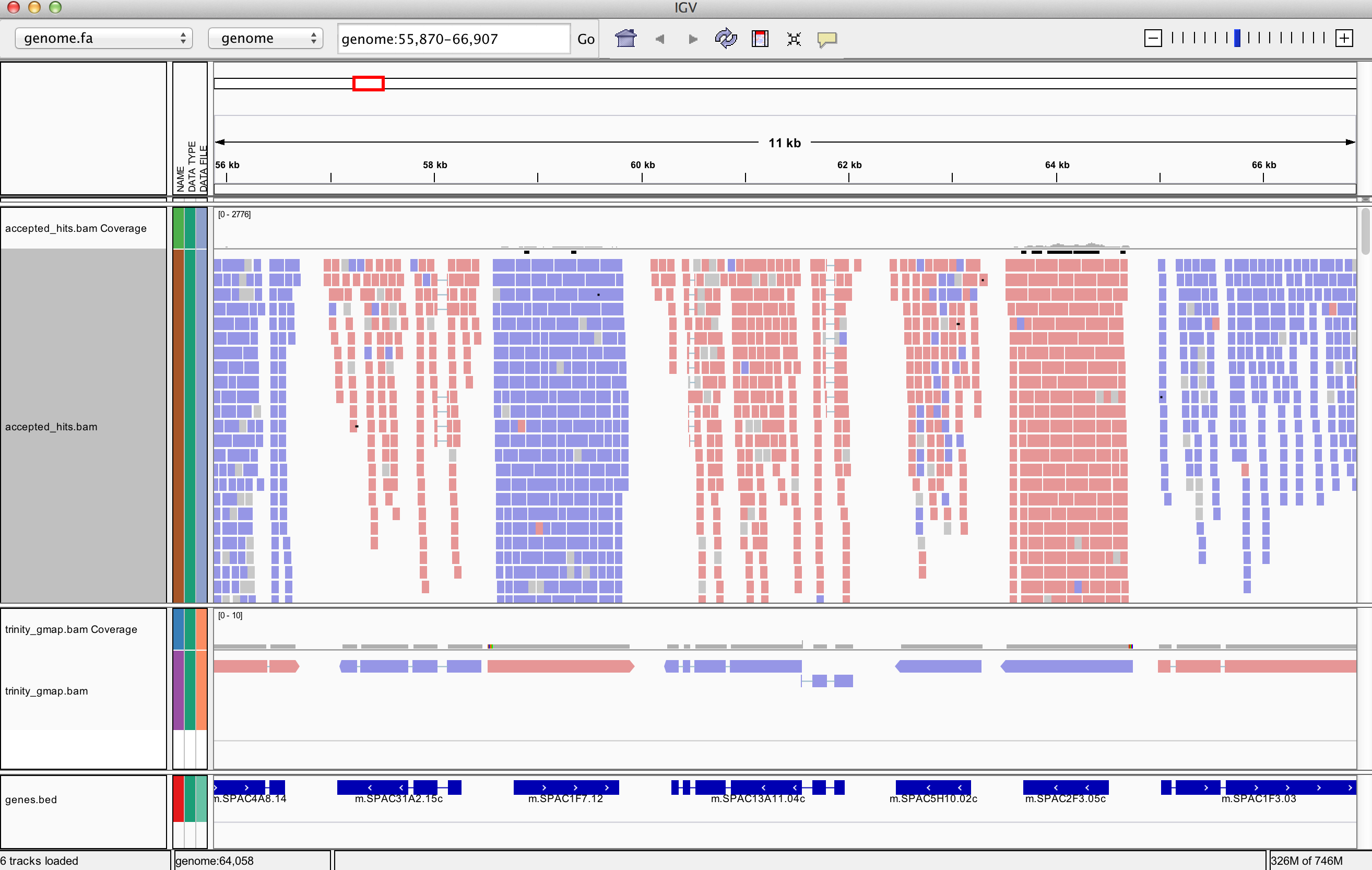
Does Trinity fully or partially reconstruct transcripts corresponding to the reference transcripts and yielding correct structures as aligned to the genome?
Are there examples where the de novo assembly resolves introns that were not similarly resolved by the alignments of the short reads, and vice-versa?
Exit the IGV viewer to continue on with the tutorial/demo.
To estimate the expression levels of the Trinity-reconstructed transcripts, we use the strategy supported by the RSEM software. We first align the original rna-seq reads back against the Trinity transcripts, then run RSEM to estimate the number of rna-seq fragments that map to each contig. Because the abundance of individual transcripts may significantly differ between samples, the reads from each sample must be examined separately, obtaining sample-specific abundance values.
For the alignments, we use ‘bowtie’ instead of ‘tophat’. There are two reasons for this. First, because we’re mapping reads to reconstructed cDNAs instead of genomic sequences, properly aligned reads do not need to be gapped across introns. Second, the RSEM software is currently only compatible with gap-free alignments.
The RSEM software is wrapped by scripts included in Trinity to facilitate usage in the Trinity framework.
The following script will run RSEM, which first aligns the RNA-Seq reads to the Trinity transcripts using the Bowtie aligner, and then performs abundance estimation. This process is
% ${TRINITY_HOME}/util/align_and_estimate_abundance.pl --seqType fq  \
      --left RNASEQ_data/Sp_ds.left.fq.gz --right RNASEQ_data/Sp_ds.right.fq.gz \
      --transcripts trinity_out_dir/Trinity.fasta \
      --output_prefix Sp_ds --est_method RSEM  --aln_method bowtie \
      --trinity_mode --prep_reference --output_dir Sp_ds.RSEM
Once finished, RSEM will have generated two files: ‘Sp_ds.isoforms.results’ and ‘Sp_ds.genes.results’. These files contain the Trinity transcript and component (the Trinity analogs to Isoform and gene) rna-seq fragment counts and normalized expression values.
Examine the format of the ‘Sp_ds.isoforms.results’ file by looking at the top few lines of the file:
% head head Sp_ds.RSEM/Sp_ds.isoforms.results
yielding (note your results may not be identical due to assembly differences):
 transcript_id	gene_id	length	effective_length	expected_count	TPM	FPKM	IsoPct
 TRINITY_DN0_c0_g1_i1	TRINITY_DN0_c0_g1	1894	1629.48	62.00	432.83	401.52	100.00
 TRINITY_DN0_c1_g1_i1	TRINITY_DN0_c1_g1	271	28.49	7.00	2795.30	2593.09	100.00
 TRINITY_DN100_c0_g1_i1	TRINITY_DN100_c0_g1	320	62.60	2.00	363.44	337.15	100.00
 TRINITY_DN100_c1_g1_i1	TRINITY_DN100_c1_g1	948	683.48	18.00	299.59	277.91	100.00
 TRINITY_DN100_c2_g1_i1	TRINITY_DN100_c2_g1	789	524.48	17.00	368.72	342.05	100.00
 TRINITY_DN101_c0_g1_i1	TRINITY_DN101_c0_g1	956	691.48	36.00	592.24	549.40	100.00
 TRINITY_DN101_c1_g1_i1	TRINITY_DN101_c1_g1	279	33.31	4.00	1365.90	1267.09	100.00
 TRINITY_DN101_c2_g1_i1	TRINITY_DN101_c2_g1	250	17.44	0.00	0.00	0.00	0.00
 TRINITY_DN102_c0_g1_i1	TRINITY_DN102_c0_g1	4736	4471.48	369.00	938.75	870.84	100.00
Quantify expression for Sp_hs:
% ${TRINITY_HOME}/util/align_and_estimate_abundance.pl --seqType fq  \
      --left RNASEQ_data/Sp_hs.left.fq.gz --right RNASEQ_data/Sp_hs.right.fq.gz \
      --transcripts trinity_out_dir/Trinity.fasta  \
      --output_prefix Sp_hs --est_method RSEM  --aln_method bowtie \
      --trinity_mode --prep_reference --output_dir Sp_hs.RSEM
.
% head Sp_hs.RSEM/Sp_hs.isoforms.results
Quantify expression for Sp_log:
% ${TRINITY_HOME}/util/align_and_estimate_abundance.pl --seqType fq  \
      --left RNASEQ_data/Sp_log.left.fq.gz --right RNASEQ_data/Sp_log.right.fq.gz \
      --transcripts trinity_out_dir/Trinity.fasta  \
      --output_prefix Sp_log --est_method RSEM  --aln_method bowtie \
      --trinity_mode --prep_reference --output_dir Sp_log.RSEM
.
% head Sp_log.RSEM/Sp_log.isoforms.results
Quantify expression for Sp_plat:
% ${TRINITY_HOME}/util/align_and_estimate_abundance.pl --seqType fq  \
      --left RNASEQ_data/Sp_plat.left.fq.gz --right RNASEQ_data/Sp_plat.right.fq.gz \
      --transcripts trinity_out_dir/Trinity.fasta  \
      --output_prefix Sp_plat --est_method RSEM  --aln_method bowtie \
      --trinity_mode --prep_reference --output_dir Sp_plat.RSEM
.
% head Sp_plat.RSEM/Sp_plat.isoforms.results
% ${TRINITY_HOME}/util/abundance_estimates_to_matrix.pl --est_method RSEM \
      --out_prefix Trinity_trans \
      Sp_ds.RSEM/Sp_ds.isoforms.results \
      Sp_hs.RSEM/Sp_hs.isoforms.results \
      Sp_log.RSEM/Sp_log.isoforms.results \
      Sp_plat.RSEM/Sp_plat.isoforms.results
You should find a matrix file called 'Trinity_trans.counts.matrix', which contains the counts of RNA-Seq fragments mapped to each transcript. Examine the first few lines of the counts matrix:
% head -n20 Trinity_trans.counts.matrix
In addition, a matrix containing normalized expression values is generated called 'Trinity_trans.TMM.EXPR.matrix'. These expression values arenormalized for sequencing depth and transcript length, and then scaled via TMM normalization under the assumption that most transcripts are not differentially expressed.
To detect differentially expressed transcripts, run the Bioconductor package edgeR using our counts matrix:
% ${TRINITY_HOME}/Analysis/DifferentialExpression/run_DE_analysis.pl \
      --matrix Trinity_trans.counts.matrix \
      --method edgeR \
      --dispersion 0.1 \
      --output edgeR
Examine the contents of the edgeR/ directory.
% ls -ltr edgeR/
.
-rw-r--r--    961 Oct 14 21:08 Trinity_trans.counts.matrix.Sp_ds_vs_Sp_hs.Sp_ds.vs.Sp_hs.EdgeR.Rscript
-rw-r--r--    965 Oct 14 21:08 Trinity_trans.counts.matrix.Sp_ds_vs_Sp_log.Sp_ds.vs.Sp_log.EdgeR.Rscript
-rw-r--r--  12089 Oct 14 21:08 Trinity_trans.counts.matrix.Sp_ds_vs_Sp_hs.edgeR.DE_results.MA_n_Volcano.pdf
-rw-r--r--  26007 Oct 14 21:08 Trinity_trans.counts.matrix.Sp_ds_vs_Sp_hs.edgeR.DE_results
-rw-r--r--    965 Oct 14 21:08 Trinity_trans.counts.matrix.Sp_hs_vs_Sp_log.Sp_hs.vs.Sp_log.EdgeR.Rscript
-rw-r--r--  12132 Oct 14 21:08 Trinity_trans.counts.matrix.Sp_ds_vs_Sp_plat.edgeR.DE_results.MA_n_Volcano.pdf
-rw-r--r--  27320 Oct 14 21:08 Trinity_trans.counts.matrix.Sp_ds_vs_Sp_plat.edgeR.DE_results
-rw-r--r--    969 Oct 14 21:08 Trinity_trans.counts.matrix.Sp_ds_vs_Sp_plat.Sp_ds.vs.Sp_plat.EdgeR.Rscript
-rw-r--r--  12359 Oct 14 21:08 Trinity_trans.counts.matrix.Sp_ds_vs_Sp_log.edgeR.DE_results.MA_n_Volcano.pdf
-rw-r--r--  27366 Oct 14 21:08 Trinity_trans.counts.matrix.Sp_ds_vs_Sp_log.edgeR.DE_results
-rw-r--r--    973 Oct 14 21:08 Trinity_trans.counts.matrix.Sp_log_vs_Sp_plat.Sp_log.vs.Sp_plat.EdgeR.Rscript
-rw-r--r--  12244 Oct 14 21:08 Trinity_trans.counts.matrix.Sp_hs_vs_Sp_plat.edgeR.DE_results.MA_n_Volcano.pdf
-rw-r--r--  26000 Oct 14 21:08 Trinity_trans.counts.matrix.Sp_hs_vs_Sp_plat.edgeR.DE_results
-rw-r--r--    969 Oct 14 21:08 Trinity_trans.counts.matrix.Sp_hs_vs_Sp_plat.Sp_hs.vs.Sp_plat.EdgeR.Rscript
-rw-r--r--  11843 Oct 14 21:08 Trinity_trans.counts.matrix.Sp_hs_vs_Sp_log.edgeR.DE_results.MA_n_Volcano.pdf
-rw-r--r--  24664 Oct 14 21:08 Trinity_trans.counts.matrix.Sp_hs_vs_Sp_log.edgeR.DE_results
-rw-r--r--  12522 Oct 14 21:08 Trinity_trans.counts.matrix.Sp_log_vs_Sp_plat.edgeR.DE_results.MA_n_Volcano.pdf
-rw-r--r--  27529 Oct 14 21:08 Trinity_trans.counts.matrix.Sp_log_vs_Sp_plat.edgeR.DE_results
The files '*.DE_results' contain the output from running EdgeR to identify differentially expressed transcripts in each of the pairwise sample comparisons. Examine the format of one of the files, such as the results from comparing Sp_log to Sp_plat:
% head edgeR/Trinity_trans.counts.matrix.Sp_log_vs_Sp_plat.edgeR.DE_results
.
logFC	logCPM	PValue	FDR
TRINITY_DN194_c0_g1_i1	9.66416591102997	14.600909190023	1.93330353190752e-20	5.915908807637e-18
TRINITY_DN200_c0_g1_i1	8.45030393326172	15.0886485738924	2.31503653655595e-19	3.5420059009306e-17
TRINITY_DN191_c0_g1_i1	7.31800087731369	16.5782506409448	3.47545039277593e-17	3.29483209332409e-15
TRINITY_DN145_c0_g1_i1	7.23267498694398	17.2926534059071	4.3069700566328e-17	3.29483209332409e-15
TRINITY_DN172_c0_g1_i1	7.71921099941212	14.0453815658946	8.07920737995993e-17	4.4830606278808e-15
TRINITY_DN160_c0_g2_i1	7.40778314235597	14.8100860739055	8.79031495662901e-17	4.4830606278808e-15
TRINITY_DN16_c0_g1_i1	7.11479775537479	15.1280266213261	3.06589559003258e-16	1.34023435792853e-14
TRINITY_DN67_c0_g2_i1	-8.07534401391914	12.7010492239743	5.72308519276669e-16	2.18908008623326e-14
TRINITY_DN243_c0_g1_i1	-11.8950563741044	12.017453198614	9.028359231807e-16	3.06964213881438e-14
These data include the log fold change (logFC), log counts per million (logCPM), P- value from an exact test, and false discovery rate (FDR).
The EdgeR analysis above generated both MA and Volcano plots based on these data. Examine any of these 'edgeR/transcripts.counts.matrix.condA_vs_condB.edgeR.DE_results.MA_n_Volcano.pdf' pdf files like so:
% evince edgeR/Trinity_trans.counts.matrix.Sp_log_vs_Sp_plat.edgeR.DE_results.MA_n_Volcano.pdf
Note, on linux, 'evince' is a handy viewer. You might also use 'xpdf' to view pdf files. On mac, try using the 'open' command from the command-line instead.

Exit the chart viewer to continue.
How many differentially expressed transcripts do we identify if we require the FDR to be at most 0.05? You could import the tab-delimited text file into your favorite spreadsheet program for analysis and answer questions such as this, or we could run some unix utilities and filters to query these data. For example, a unix’y way to answer this question might be:
% sed '1,1d' edgeR/Trinity_trans.counts.matrix.Sp_log_vs_Sp_plat.edgeR.DE_results | awk '{ if ($5 <= 0.05) print;}' | wc -l
.
69
Trinity facilitates analysis of these data, including scripts for extracting transcripts that are above some statistical significance (FDR threshold) and fold-change in expression, and generating figures such as heatmaps and other useful plots, as described below.
Now let's perform the following operations from within the edgeR/ directory. Enter the edgeR/ dir like so:
% cd edgeR/
Extract those differentially expressed (DE) transcripts that are at least 4-fold differentially expressed at a significance of <= 0.001 in any of the pairwise sample comparisons:
% $TRINITY_HOME/Analysis/DifferentialExpression/analyze_diff_expr.pl \
                --matrix ../Trinity_trans.TMM.EXPR.matrix -P 1e-3 -C 2
The above generates several output files with a prefix “diffExpr.P1e-3_C2”, indicating the parameters chosen for filtering, where P (FDR actually) is set to 0.001, and fold change (C) is set to 2^(2) or 4-fold. (These are default parameters for the above script. See script usage before applying to your data).
Included among these files are: ‘diffExpr.P1e-3_C2.matrix’ : the subset of the FPKM matrix corresponding to the DE transcripts identified at this threshold. The number of DE transcripts identified at the specified thresholds can be obtained by examining the number of lines in this file.
% wc -l diffExpr.P1e-3_C2.matrix
.
57
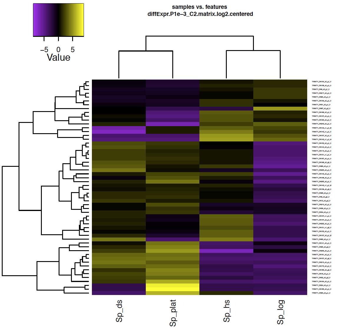
Note, the number of lines in this file includes the top line with column names, so there are actually 56 DE transcripts at this 4-fold and 1e-3 FDR threshold cutoff.
Also included among these files is a heatmap ‘diffExpr.P1e-3_C2.matrix.log2.centered.genes_vs_samples_heatmap.pdf’ as shown below, with transcripts clustered along the vertical axis and samples clustered along the horizontal axis.
% evince diffExpr.P1e-3_C2.matrix.log2.centered.genes_vs_samples_heatmap.pdf
Exit the PDF viewer to continue.
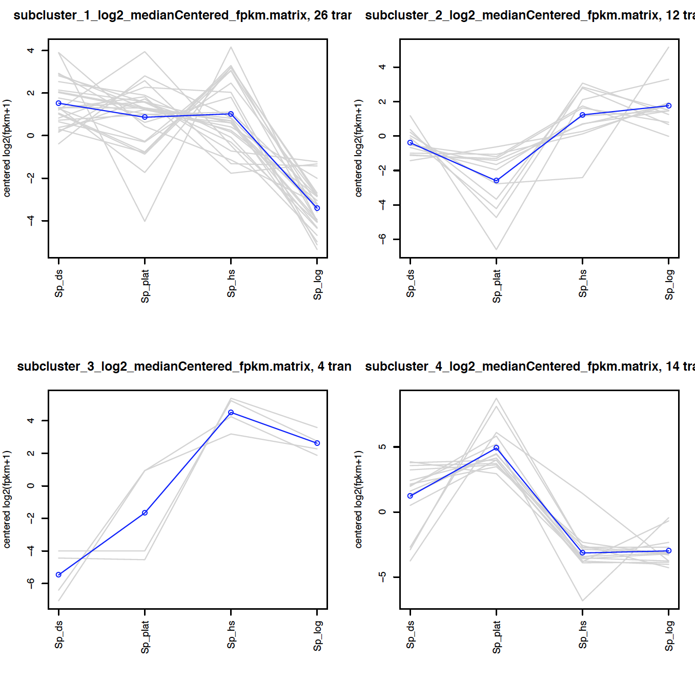
Extract clusters of transcripts with similar expression profiles by cutting the transcript cluster dendrogram at a given percent of its height (ex. 60%), like so:
% $TRINITY_HOME/Analysis/DifferentialExpression/define_clusters_by_cutting_tree.pl \
       --Ptree 60 -R diffExpr.P1e-3_C2.matrix.RData
This creates a directory containing the individual transcript clusters, including a pdf file that summarizes expression values for each cluster according to individual charts:
% evince diffExpr.P1e-3_C2.matrix.RData.clusters_fixed_P_60/my_cluster_plots.pdf
More information on Trinity and supported downstream applications can be found from the Trinity software website: http://trinityrnaseq.github.io