kriging (v2.3)

Ordinary and universal kriging in N dimensions.

kriging is a basic implementation of kriging, a method of interpolation using Gaussian process regression. kriging supports ordinary kriging and universal kriging (using a polynomial drift term), and several variogram models.

In the presence of drift (a varying mean value across the data space), the observed variogram can be biased (see Starks & Fang, 1982, Mathematical Geology, 14, 4; https://doi.org/10.1007/BF01032592). kriging attempts to remove this bias by subtracting a fitted polynomial drift term before generating the variogram.

kriging also handles data uncertainties and covariances. If the data have associated errors, then the data variances and covariances are factored into the kriging system of equations (see, for example, Cecinati et al., 2018, Atmosphere, 9(11), 446; https://doi.org/10.3390/atmos9110446).

Installation

Install directly from this repository:

pip install git+https://github.com/tvwenger/kriging.git

Or, clone the repository and:

python setup.py install

Usage

from kriging import kriging
krig = kriging.Kriging(obs_pos, obs_data, e_obs_data=e_obs_data, obs_data_cov=obs_data_cov)
variogram_fig = krig.fit(
    model=model, deg=deg, nbins=nbins, bin_number=bin_number, lag_cutoff=lag_cutoff)
interp_data, interp_var = krig.interp(interp_pos, resample=resample)

Functions & Arguments:

Object Initialization

Intialize a new Kriging object.

krig = kriging.Kriging(obs_pos, obs_data, e_obs_data=e_obs_data, obs_data_cov=obs_data_cov)

• obs_pos is the NxM scalar array of the N observed Cartesian positions in M dimensions.
• obs_data is the N-length scalar array of observations at each position.
• e_obs_data (optional) is the N-length scalar array of observed value uncertainties (standard deviation). If None (default), then the data covariance matrix can be supplied via obs_data_cov. If both are None, then data uncertainies are not considered in the kriging solution.
• obs_data_cov (optional) is the NxN scalar array of observed data covariances. If None (default), then the (uncorrelated) data uncertainties can be supplied via e_obs_data. If both are None, then data uncertainies are not considered in the kriging solution.

Fitting a Variogram Model

Fit and remove a polynomial drift component and then fit a variogram model to the drift-subtracted data.

variogram_fig = krig.fit(
    model=model, deg=deg, nbins=nbins, bin_number=bin_number, lag_cutoff=lag_cutoff, plot=plot)

• model (optional) is the assumed variogram model. Available values can be found via: from kriging import kriging; print(kriging._MODELS.keys())
• deg (optional) is the degree of the polynomial drift term. deg=0 (default) is equivalent to ordinary kriging (no drift).
• nbins (optional) is the number of lag bins to use when generating the variogram. The default value is 6.
• bin_number (optional) is a flag to set how the lag bins are spaced. The default value is False, which means that the lag bins have equal width covering the full range of observed lags. If True, then each lag bin includes the same number of data.
• lag_cutoff (optional) is the maximum lag used to fit the variogram relative to the maximum separation of the observed data. The value of this parameter should be between 0.0 (not inclusive) and 1.0 (inclusive, default).
• plot (optional) if True, generate and return variogram model plot.
• variogram_fig (optional) fitted variogram model plot (gammavariance vs. lag). Value is None if plot=False.

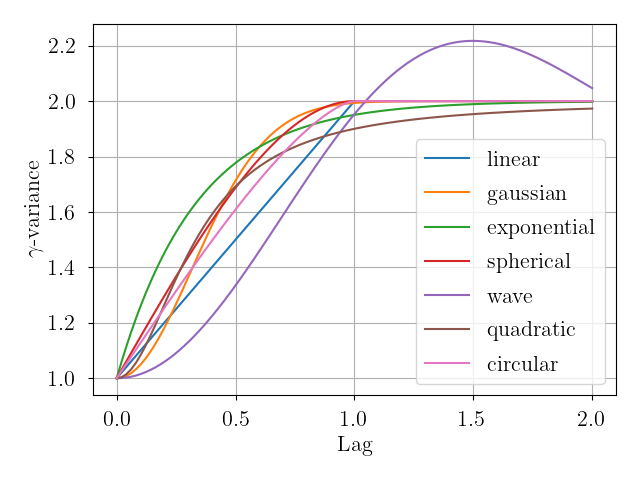
Here is a visual representation of the available variogram models, each having parameters nugget = 1.0, sill = 1.0, and range = 1.0.

Interpolation

Solve the kriging system of equations and evaluate the interpolation and variance a given positions.

interp_data, interp_var = krig.interp(interp_pos, resample=resample)

• interp_pos is the LxM scalar array of L Cartesian positions at which to calculate interpolated values.
• resample (optional) is a flag to use resampled observed data to solve the kriging system of equations. The observed data samples are drawn from a multivariate normal distribution defined by the observed data covariance matrix.
• interp_data is the L-length scalar array of interpolated values at each interp_pos position.
• interp_var is the L-length scalar array of variances at each interp_pos position.

Example

For more examples, see the notebooks in the example directory.

Universal Kriging

import numpy as np
import matplotlib.pyplot as plt
from kriging import kriging

# set a random seed for reproduciblity
np.random.seed(1234)

# the "true" field
def truth(pos):
    # pos = (N, M) array of N scalar positions in M dimensions
    # true field is a horizontal gradient + Gaussian ring
    horiz_gradient = 0.5
    data = horiz_gradient * pos[:, 0]
    radius = np.sqrt((pos**2.0).sum(axis=1))
    ring_amp = 10.0
    ring_rad = 8.0
    ring_sig = 2.0
    data += ring_amp * np.exp(-0.5 * ((radius - ring_rad)/ring_sig)**2.0)
    return data

# interpolation grid
xgrid, ygrid = np.mgrid[-15:15:100j, -15:15:100j]
extent = [xgrid.min(), xgrid.max(), ygrid.min(), ygrid.max()]
grid_pos = np.vstack((xgrid.flatten(), ygrid.flatten())).T

# plot "truth"
true_data = truth(grid_pos)
plt.imshow(true_data.reshape(xgrid.shape).T, origin='lower', extent=extent, vmin=-10, vmax=15)
plt.colorbar(label="Truth")
plt.tight_layout()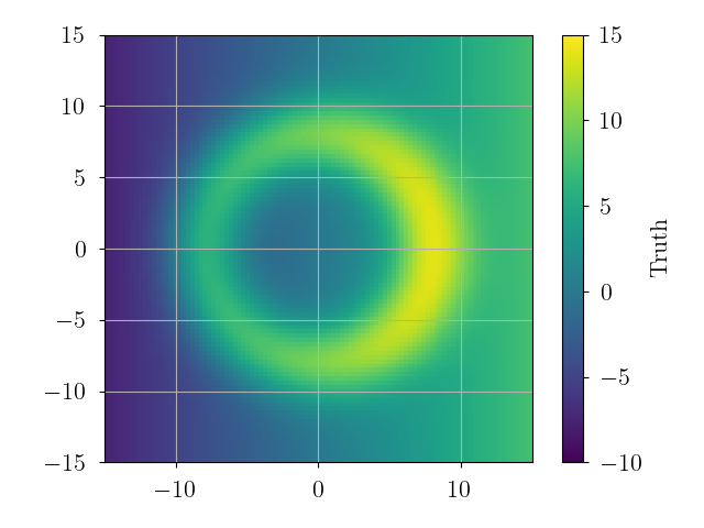

# randomly sample observations of the "true" field
num_data = 100
obs_pos = np.random.uniform(-15.0, 15.0, size=(num_data, 2))
obs_data = truth(obs_pos)

# add some Gaussian noise
e_obs_data = 1.0 * np.ones(len(obs_data))
obs_data += e_obs_data * np.random.randn(len(obs_data))

# universal kriging (deg=1)
krig = kriging.Kriging(obs_pos, obs_data, e_obs_data=e_obs_data)
variogram_fig = krig.fit(
    model="wave", deg=1, nbins=10, bin_number=False, lag_cutoff=0.5)
interp_data, interp_var = krig.interp(grid_pos)
variogram_fig.show()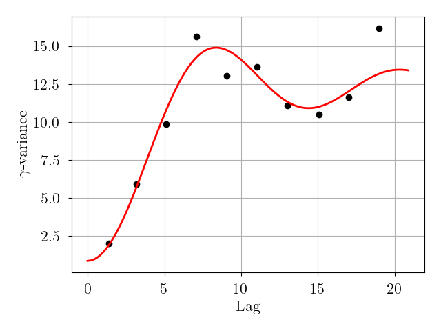

# plot interpolation
plt.imshow(interp_data.reshape(xgrid.shape).T, origin='lower', extent=extent, vmin=-10.0, vmax=15.0)
plt.scatter(obs_pos[:, 0], obs_pos[:, 1], c=obs_data, edgecolor='k', marker='o', vmin=-10.0, vmax=15.0)
plt.colorbar(label="Interpolation")
plt.show()

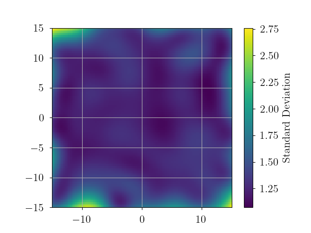
# plot standard deviation
interp_std = np.sqrt(interp_var)
plt.imshow(interp_std.reshape(xgrid.shape).T, origin='lower', extent=extent)
plt.colorbar(label="Standard Deviation")
plt.show()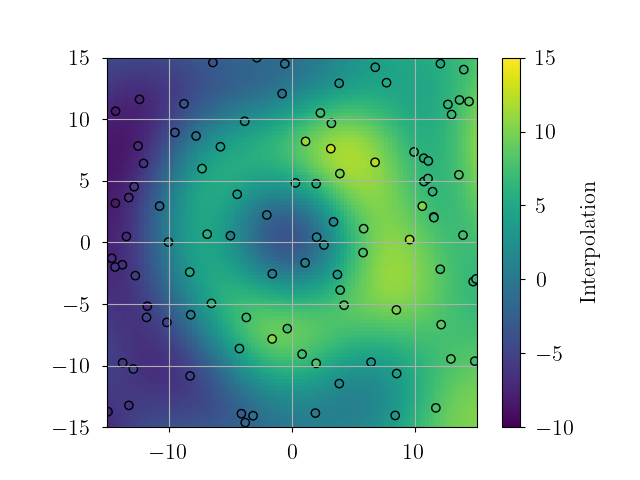

Issues and Contributing

Please submit issues or pull requests via Github.

License and Warranty

GNU General Public License v3 (GNU GPLv3)

This program is free software: you can redistribute it and/or modify it under the terms of the GNU General Public License as published by the Free Software Foundation, either version 3 of the License, or (at your option) any later version.

This program is distributed in the hope that it will be useful, but WITHOUT ANY WARRANTY; without even the implied warranty of MERCHANTABILITY or FITNESS FOR A PARTICULAR PURPOSE. See the GNU General Public License for more details.

You should have received a copy of the GNU General Public License along with this program. If not, see http://www.gnu.org/licenses/.