Decoding with ERPLAB Studio
Now that you’ve learned about the essence of decoding, it’s finally time to see how you can actually decode data in ERPLAB Studio. We’re going to focus on how to perform decoding using ERPLAB Studio’s GUI, but each step can also be scripted. As usual, ERPLAB's history will include the script equivalent of every routine that you run in the GUI (which you can access from the History panel). A great way to learn scripting is to start by doing decoding in the GUI and then use the script equivalents to start building a decoding script.
In this tutorial, we’ll be decoding the four face identities and the four emotion expressions from the study of Bae (2021), focusing on the data from 5 of the participants. You can download the data at https://doi.org/10.18115/D5KS6S. Keep in mind that these data have been filtered with a half-amplitude low-pass cutoff at 20 Hz, whereas the Bae (2021) study used a cutoff of 6 Hz. A 6 Hz cutoff helps reduce trial-to-trial variability due to alpha-band EEG oscillations, but it also reduces your temporal resolution. It’s great for looking at sustained activity in working memory, but a 20 Hz cutoff is more appropriate for most purposes.
ERPLAB’s decoding is designed to be very simple if you already know how to do conventional ERP processing using ERPLAB (in combination with EEGLAB). You use BINLISTER to define your classes and then perform a few extra steps, and you’re done! For example, we’ll create separate bins for each of the four face IDs, collapsed across emotion expressions, and we’ll decode those bins/classes. We’ll also create separate bins for each of the four emotion expressions, collapsed across face ID, and then we’ll decode those bins/classes.
I’m assuming that you already understand the basics of using ERPLAB Studio for conventional ERP analyses. If you don’t already have a thorough understanding, including BINLISTER, I recommend that you go through the ERPLAB Studio Tutorial before proceeding further with this decoding tutorial.
Important note: Versions of Matlab prior to 2023b use a virtual machine to run on Apple computers that have Apple processors (e.g., the M1 and M2 processors). This can be slow (especially launching GUI windows) and Matlab often crashes (especially during plotting). We recommend using Matlab 2023b or later if you have a computer with “Apple silicon”.
Here's a brief overview of the steps involved in ERPLAB’s decoding pipeline:
- Preprocess the continuous EEG data in the EEG tab just as you would for a conventional ERP analysis, including filtering and artifact correction. The location of the reference location doesn’t have much impact on decoding accuracy, so any reference is fine. If you have any bad channels, you can either delete them (using the Edit/Delete Channels & Locations panel) or interpolate them (using the Interpolate Channels panel).
- Use the Assign Events to Bins (BINLISTER) panel to sort your trials into the classes you want to decode. Each bin will be a different class. It’s up to you to decide how your classes/bins are defined. For example, you could include only trials with correct behavioral responses, only trials with a behavioral response within a particular time window, etc. These decisions are based on the specific scientific hypotheses you are testing, so we can’t provide any general advice about how to define your classes/bins.
- Convert the continuous EEG data into discrete epochs (e.g., -500 to +1500 ms) using the Extract Bin-Based Epochs panel.
- Perform artifact detection using the Artifact Detection panel if desired. Remember, trial-to-trial variability is the enemy of decoding accuracy, so eliminating epochs with large voltage deflections in any channel is usually a good idea. However, you will need to “floor” the number of trials across classes (and possibly across conditions or groups), and decoding accuracy declines as the number of trials declines, so it can be a problem to reject too many trials. As usual, it’s best to minimize artifacts during recording rather than dealing with them after they’ve already contaminated your data (Hansen’s Axiom: There is no substitute for clean data).
- Export the epoched EEG as a set of bin-epoched single trials (a BESTset) using the Extract Bin-Epoched Single Trials (BEST) panel. This is not a typical step in ERP processing, but it is a necessary step in our decoding pipeline. A BESTset is just a reorganized version of an epoched EEGLAB .set file that is particularly convenient for the cross-validation procedure that is a key part of decoding. When you save the BESTset, you should exclude any trials that were marked for rejection. When you create the BESTset, you can convert the data from voltage into phase-independent activity within a given frequency band (using the Hilbert transform). For example, you can specify a frequency band of 8-12 Hz to convert the voltage into alpha-band activity, allowing you to perform decoding in the frequency domain (see Bae & Luck, 2018, for details). When the BESTsets are created, they appear in the BESTsets panel in the Pattern Classification tab.
- Perform decoding on the BESTset using the Multivariate Pattern Classification panel in the Pattern Classification tab. You can apply this tool to multiple BESTsets (one per subject) at the same time. That makes it easier to floor the number of trials across subjects, if desired. The output for each BESTset is a data structure called an MVPCset, which appears in the MVPCsets panel. MVPCsets can be saved to disk with a filename extension of .mvpc. An MVPCset contains the decoding accuracy values and other useful information.
- View a plot of the decoding accuracy, which automatically appears in the ERPLAB Studio plot region when an MVPCset is created or selected. If multiple MVPCsets are selected, they are overlaid in the same plot. You can control the plotting parameters (e.g., the X and Y scales) using the Plot Settings (MVPCsets) panel. You can save the plots in several different formats by going to the Plotting Options menu under the plot region and selecting Save Figure as.
- You can plot the “confusion matrix” for each selected MVPCset using the Plot Confusion Matrices panel. This is used when you have more than two classes, allowing you to get more information about the pattern of errors. For example, when the true class was face ID 1, the confusion matrix will show you how often the decoder guessed ID 1, verus ID 2 versus ID 3 versus ID 4.
- Average decoding accuracy across participants using the Average Across MVPCsets (Grand Average) panel. This creates a new MVPCset that is the average across all the selected MVPCsets. It will automatically be plotted in the ERPLAB Studio plot region.
- Export the decoding accuracy at each time point to a text file using the Export button in the MVPCsets panel. This file can then be imported into a spreadsheet or statistical analysis program for further analyses.
The following subsections will explain each of these steps in more detail and show you how to implement them with the data from the first five subjects in the study of Bae (2021).
Let’s start by opening the continuous EEG from subject 301 by going to the EEGsets panel in the EEG tab, clicking Load, and navigating to the file named 301_preprocessed.set. You should scroll through the data to make sure everything looks reasonable. Note that the file begins with approximately 18 seconds of EEG data before the first event codes (which provides a buffer to minimize edge artifacts during filtering).
These data have already undergone several preprocessing steps, including filtering with a half-amplitude bandpass of 0.1 to 80 Hz and re-referencing to the average of the left and right mastoids (see Bae (2021) for a list of all the preprocessing steps). In addition, an EVENTLIST was added to this EEGset, and a low-pass filter with a half-amplitude cutoff at 20 Hz was applied.
We now need to use BINLISTER to assign the events to bins. The following table shows what each event code means. We have 16 different stimulus codes, each representing one combination of the 4 face IDs and the 4 emotion expressions.
| Face ID 1 | Face ID 2 | Face ID 3 | Face ID 4 | |
|---|---|---|---|---|
| Fearful | 211 | 212 | 213 | 214 |
| Happy | 221 | 222 | 223 | 224 |
| Neutral | 231 | 232 | 233 | 234 |
| Angry | 241 | 242 | 243 | 244 |
We are going to do two separate sets of decoding analyses, one in which we decode face identity irrespective of emotion expression and one in which we decode emotion expression independent of face identity. For the face identity decoding, we want one bin for each of the four face identities, ignoring the emotion expression. For face ID 1, this would be event codes 211, 221, 231, and 241. For the emotion expression decoding, we want one bin for each of the four emotion expressions, ignoring the face identity. For the fearful expression, this would be event codes 211, 212, 213, and 214. Thus, we want a total of 8 bins, with the first 4 being used to decode face identity and the last 4 being used to decode emotion expression. The file named BDF_ID_Expression.txt is used to define these 8 bins. I recommend opening the file to make sure you understand how it works.
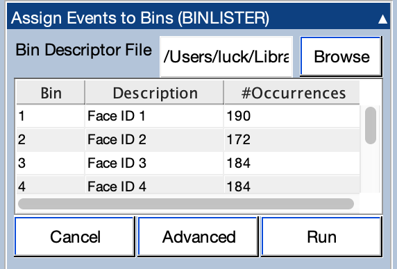
To sort the event codes into bins in this manner, go to the Assign Events to Bins (BINLISTER) panel and tell it to use BDF_ID_Expression.txt as the bin descriptor file. Click Run, and then use the recommended name for the new EEGset (301_preprocessed_bins). Once BINLISTER is done running, you will be able to see the number of event codes in each bin in the table within the panel (see screenshot below). You'll need to scroll within the table to see all 8 bins.
The next step is to take the continuous EEG and break it into epochs. We’ll use an epoch length of -200 to +800 ms (i.e., from 200 ms before stimulus onset to 800 ms after stimulus onset). To do this, go to the Extract Bin-Based Epochs panel, enter -200 800 in the Time Range box, and make sure the Baseline Period is set to Pre. Click Apply and use the recommended EEGset name (301_preprocessed_bins_be). You might want to save the resulting dataset to disk so that you can recover it if you need to quit from EEGLAB.
You should now see the epoched EEG data in the plot region.
Ordinarily, the next step would be to apply artifact detection to mark epochs with large voltage deflections arising from skin potentials, movement, muscle contractions, etc. However, the EEGsets we're analyzing in this tutorial were exceptionally clean, so we will skip that step.
Our next step is to create a BESTset, which is a special format for the single-trial epochs we extracted in the last step. Make sure that dataset is loaded and is the active dataset (301_preprocessed_bins_be). To create the BESTset, open the Extract Bin-Epoched Single Trials (BEST) panel. The screenshot shows what it should look like.
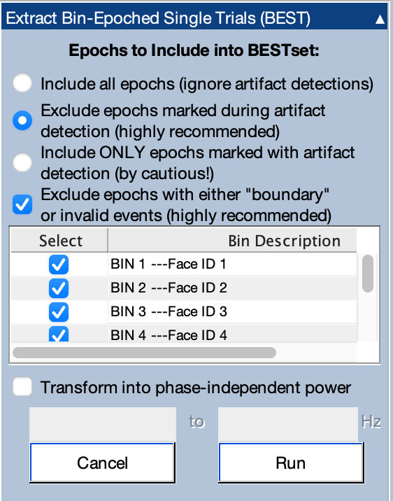
The top portion of the panel allows you to determine what to do with epochs containing artifacts and boundary events. Ordinarily, you will want to exclude epochs that were marked during artifact detection. We didn’t do any artifact detection, but we can leave that selected. You will also want to exclude any epochs that contain boundary events or other kinds of invalid events. Those epochs are probably corrupted.
The table in the middle of the panel shows the available bins. You could create a BESTset using a subset of the available bins, but we’re going to use all 8 bins, so make sure that the boxes are checked for all bins.
You also have the option of using the Hilbert transform to convert the voltages into phase-independent power within a specified frequency band (e.g., 8-12 Hz for alpha). We won’t use this option in the present tutorial.
Once you’ve made sure that the settings match those in the screenshot, click Run to proceed.
You should tell it to use 301 (the participant ID number) as the BEST name. It’s also a good idea to save it to disk.
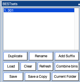
Once the BESTset is created, ERPLAB Studio will switch to the Pattern Classification tab, and you'll be able to see the new BESTset in the BESTsets panel (see screenshot below).
You might be wondering what a BESTset is and why we use it. It’s basically a convenient way of organizing the data from an epoched EEGLAB dataset structure. Whereas the dataset structure contains the EEG epochs in a somewhat complicated format, ordered by trial number, a BESTset pulls out the data from each bin into a 3-dimensional matrix with dimensions of electrode site, time point, and trial number. These matrices are much simpler and more efficient to access. This simplicity and efficiency is very helpful for the cross-validation process used in ERPLAB’s decoding pipeline.
Just like datasets and ERPsets, multiple BESTsets can be loaded into memory. You can see and select them from the BESTsets panel. There should be only one loaded at this moment. However, each BESTset you create will be added to this list. This panel also allows you to load previously saved BESTsets from your hard drive, rename the BESTsets, etc. You can also access the current BESTset and the entire set of loaded BESTsets in the BEST and ALLBEST variables in the Matlab workspace.
If you know at least a little about Matlab programming, I recommend double-clicking on the BEST variable in the Matlab workspace so that you can see how this data structure is organized. The structure is shown in the screenshot. Most of the fields are pieces of “header” information that indicate things like the sampling rate, the number of bins, the number of channels, etc. Most of these variables correspond to variables in the EEG structure used to store datasets.


The actual data are stored in BEST.binwise_data. For the present BESTset, this structure contains 8 elements, one for each bin, with each bin organized as an array of channels x time points x trials. [It can’t be a single 4-dimensional array because the number of trials is not the same across bins.] As shown in the screenshot, we have 67 channels x 250 time points x somewhere between 172 and 190 trials per bin.
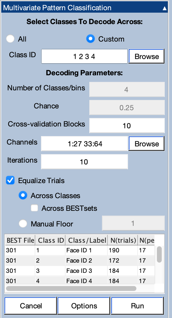
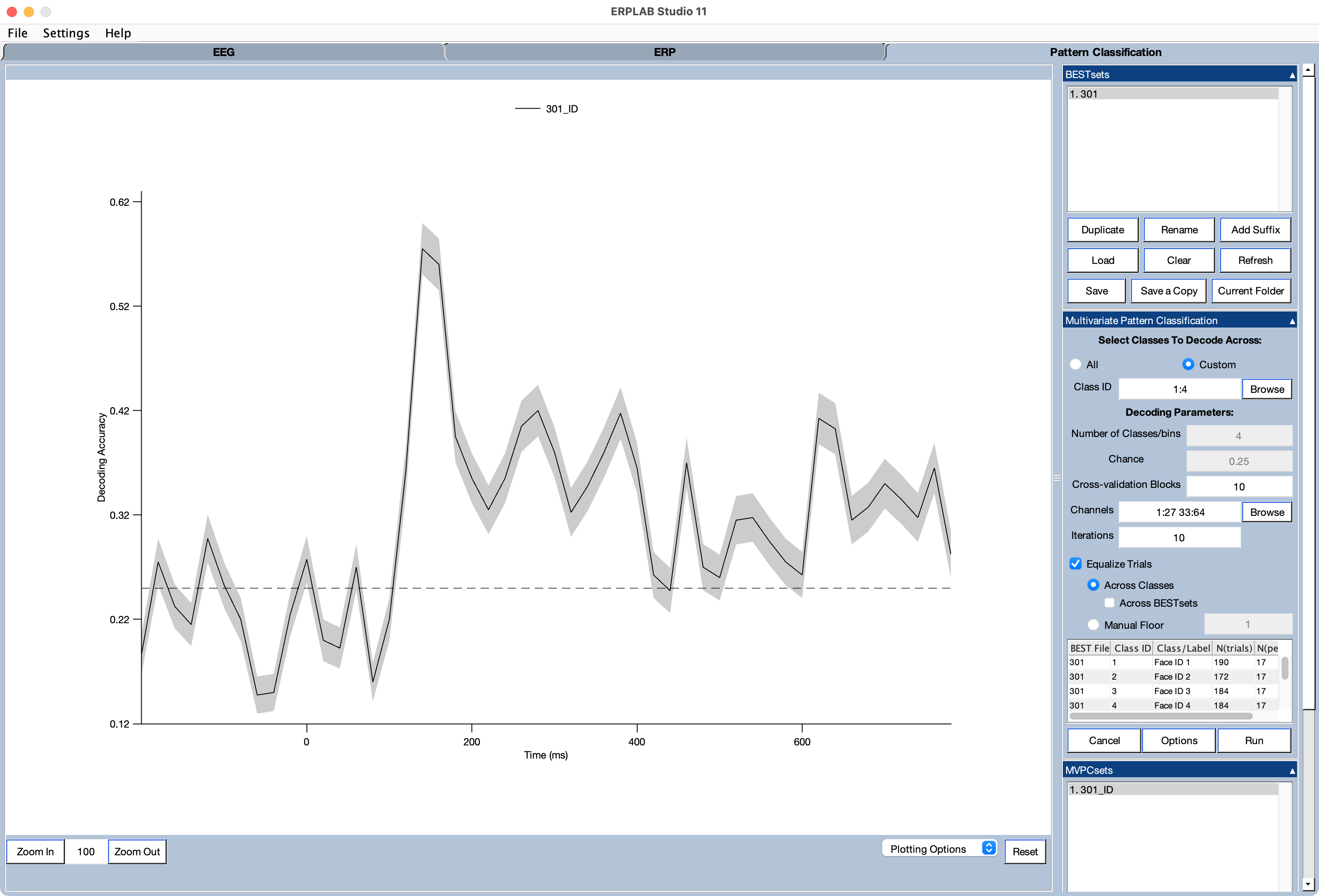
We’re finally ready to start the actual decoding! To do this, make sure that the BESTset from the previous step (301) is the active BESTset in the BESTsets panel and then go to the Multivariate Pattern Classification panel. Once we've set the parameters, it will look like the screenshot below.
First we need to decide which bins to feed into the decoder. Each bin is a class, so the bins we choose will determine the nature of the classification that will be performed.
If you look at the panel near the bottom of the panel, you'll see a list of the available bins in the selected BESTset. We’re going to start by decoding face identity, so we want to use only classes 1, 2, 3, and 4. We specify this in the area of the panel labeled Select Classes to Decode Across by changing it from All to Custom and putting 1 2 3 4 in the Class ID field (or, alternatively, 1:4, which is Matlab’s way of specifying all values between 1 and 4).
We also want to limit the decoding to the scalp EEG channels, leaving out the artifact channels, mastoids, and especially the photosensor channel. We can do this by clicking on the Browse button next to where it says Channels. That brings up a window showing the available channels. You should select the EEG channels. When you click OK, this puts the channel numbers in the text box (1:27 33:64).
We need to determine the number of cross-validation folds, which is the same thing as the number of averages that will be created for each class and the number of trials per average. We currently recommend aiming for 10-20 trials per average. As you can see from the column labeled N(trials) inside the table in the panel, we have between 172 and 190 trials per class, so 10 cross-validation blocks will give us approximately 17 trials per average. Go ahead and put 10 in the text box for Cross-Validation Blocks. You can now see that there will be 17 trials per average in the column of the table labeled N(per ERP).
The box labeled Equalize Trials is checked by default. This “floors” the number of trials. The option for flooring Across Classes should be set. This causes the number of trials per average to be the same for all classes. The smallest number of trials in a class was 172, and with 10 averages (crossfolds), this gives us 17 trials per average. The algorithm will grab a random 17 trials for each average (without replacement), and a few trials are typically unused to achieve exactly the same number of trials per average (e.g., 170 of the 172 trials will be used for Class 2). Different random subsets of trials are used on each iteration of the decoding procedure, so all trials are eventually used.
If we had multiple BESTsets loaded, we could also tell the algorithm to use the same floor across all the BESTsets. In other words, it would find the combination of class and BESTset with the lowest number of trials and use that to calculate the number of trials to be used for all classes and all BESTsets. That’s usually appropriate only when you are looking at individual differences or group differences in decoding accuracy and you don’t want decoding accuracy to be influenced by the number of trials. If you are doing a completely within-subjects manipulation, you don’t usually need to floor across BESTsets.
It's also possible to set an arbitrary floor using the Manual Floor option. For example, imagine that you are doing one run of decoding for Condition A and another run of decoding for Condition B. If you will be comparing decoding accuracy across Conditions A and B, you want to make sure that the same number of trials is used in these two conditions. You can figure out the lowest number of trials that works for all classes in both conditions and use this as the floor. But the number of trials must be small enough that the number of trials multiplied by the number of averages (i.e., the number of cross-validation blocks) does not exceed the number of trials.
Near the beginning of this tutorial, I said that there were 40 trials for each of the 16 combinations of face ID and emotion expression. That should give us 160 trials for each face ID after collapsing across emotion expressions (and 160 trials for each emotion expression after collapsing across face ID). However, the number of trials in each class shown in the decoding GUI for subject 301 ranges from 172–190. The other subjects have exactly 160 trials in each of these classes. I’m not sure of this, but I suspect that the stimulus presentation program was updated after the first subject to achieve exactly 40 trials per image. With the 10-fold cross-validation we are using, the other subjects will have 16 trials per average. You could achieve this number of trials per average with subject 301 by selecting the Manual Floor option with a floor of 16 trials.
The remaining text box is labeled Iterations, and it determines how many iterations are tested. We usually use 100, but for the sake of time, you should enter 10 for this tutorial.
Now click the Options button to see the available decoding options. You will see a window like the one shown in the screenshot below.
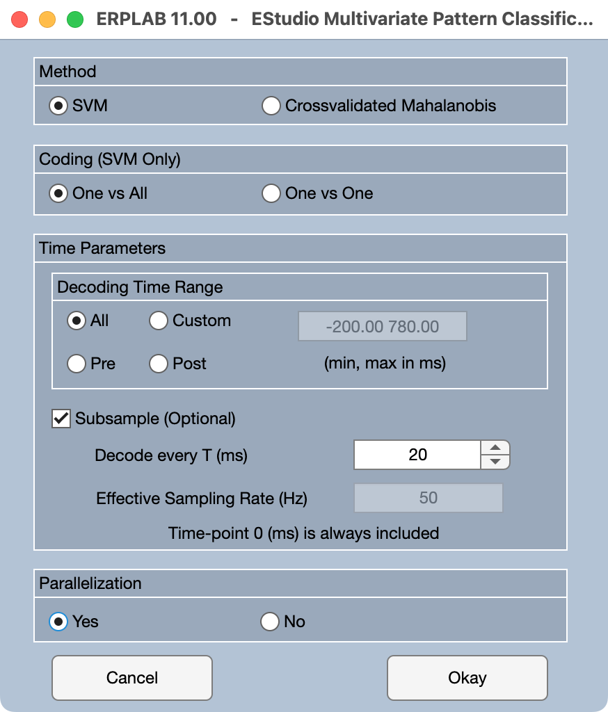
We currently implement two different multivariate pattern classification algorithms, support vector machines (SVMs) and the cross-validated Mahalanobis distance (crossnobis distance). This tutorial focuses on decoding using SVMs, so SVM should be selected as the Method.
As described earlier in the tutorial, there are two ways of doing SVM-based decoding when you have more than two classes. In 1-versus-1 decoding, a separate decoder is trained for each pair of classes (e.g., Class 1 versus Class 2; Class 1 versus Class 3; etc.). In 1-versus-all decoding, a separate decoder is trained for each class relative to the combination of the other classes (e.g., Class 1 versus Classes 2, 3, and 4; Class 2 versus Classes 1, 3, and 4; etc.). Our lab generally finds that the 1-versus-all approach works best, so you should select One vs All.
The remaining options impact how long it takes the decoding to run. With many cross-validation folds, many iterations, and many time points, it can take hours or days to decode the data from all the participants in an experiment. When you’re first learning to decode, you don’t want to wait that long to see if things have worked. In addition, when you’re doing a preliminary set of analyses, you might not want to spend hours or days on the decoding.
One key factor that impacts the amount of time is the number of time points. There are two ways to influence this. One is the Decoding Time Range. If you have very long epochs, you might not want to decode the entire time range. For example, if your epoch goes from -500 to +1500 ms, but most of the “action” is in the first 500 ms, you might want to do your initial decoding from -100 to +500 ms. (It’s a good idea to include at least 100 ms of the prestimulus interval so that you can verify that decoding is near chance during this interval. If it’s not, then that’s a strong hint that something is wrong.) Our epoch is only -200 to +800, so we’ll select All for the time range.
The other way to impact the number of time points is to only decode every Nth time point. The present BESTset is sampled at 250 Hz, which means that there is one time point every 4 ms. For an initial attempt at decoding, let’s decode every 5th time point (one time point every 20 ms). We can accomplish this by setting Decode every T (ms) to 20. This reduces our temporal resolution, but that’s OK for an initial test run.
A third factor that controls the amount of time is the Parallelization option near the bottom of the panel. When this is turned on, Matlab will see how many processing cores are in your CPU and attempt to use most of them. This can really speed up the decoding (although it might slow down other things you are trying to do on your computer while you’re decoding). However, it may take several seconds for Matlab to get the cores set up once you start decoding. This option requires that “Parallel Computing Toolbox” is already installed in MATLAB.
Once you have set all the options, click Okay.
Once you have entered all the parameters as described above, you can click the Run button in the Multivariate Pattern Classification panel. This will bring up a GUI window allowing you to name the output structure (the MVPCset) that will store the decoding accuracy values and save it as a file (see screenshot). By default, it will use the BESTset name as the MVPCset name. However, you can edit the MVPCset name. Let’s use 301_ID as the MVPCset name to indicate that we are decoding face ID rather than emotion expression. You can also tell it to use the MVPCset name as the filename (which I recommend because it will avoid confusion later).
For this tutorial, you should check the box for saving the MVPCset to disk, and you should use the MVPCset name (301_ID) as the filename. Then click the Okay button to start the decoding process.
If you have selected Parallelization, Matlab may spend several seconds allocating the processor cores before anything happens. Once the decoding is running, you’ll be able to see which iteration is currently running by looking at the status region at the bottom of the ERPLAB Studio window.
The decoding might take several minutes to complete. If you need to terminate the decoding process before it finishes, go to the Matlab Command Window at press control-C on your keyboard.
Once the decoding finishes, it creates an MVPCset, which is shown in the MVPCsets panel. The decoding accuracy is also shown in the plot region. This is shown in the screenshot below. If desired, you can control the plotting using the Plot Settings (MVPCsets) panel. You can save the plot as a file (in several different formats) by going to the Plotting Options menu near the bottom of the ERPLAB Studio window and selecting Save Figure as.
The decoding routine creates an MVPCset to store the decoding results. Multiple MVPCsets can be held in memory at a given time and can be accessed either with the MVPCsets panel or with the MVPC and ALLMVPC variables in the Matlab workspace.
The decoding accuracy values can be saved in a text file by clicking the Export button in the MVPCsets panel. This text file is easily imported into Excel and most statistics packages. When you click Export, you will see the window of options shown below.
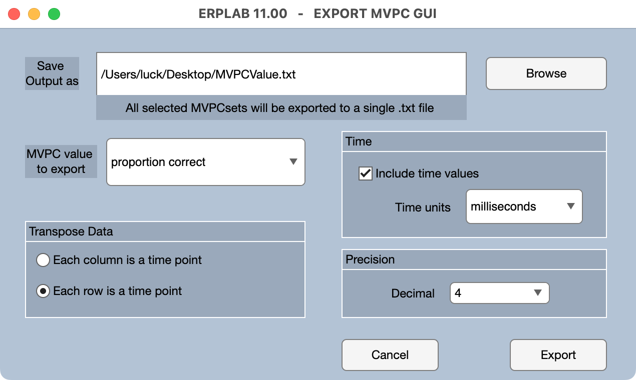
You can have a separate row for each MVPCset and a separate column for each time point (Each column is a time point) or a separate column for each MVPCset and a separate row for each time point (Each row is a time point).
You can also choose whether to Include time values for each time point in the output file and the Precision used to print the time values and decoding accuracy values (i.e., the number of digits to the right of the decimal point).
Once you have performed the decoding across multiple participants, creating a separate MVPCset for each participant, you can make a grand average MVPCset by averaging across the single-participant MVPCsets. This is accomplished using the Average Across MVPCsets (Grand Average) panel.
The result is just another MVPCset. The only difference is that the standard error values in the MVPCset indicate the standard error of the mean across participants (calculated as SD÷sqrt[N]) rather than the standard error of the single-participant decoding accuracy (calculated using the properties of a binomial distribution).
To see how this works, let’s look at the decoding results for all five participants in the provided data. You can either repeat the decoding process for each participant or you can load in the pre-made MVPCsets in the MVPCsets folder using the MVPCsets panel. If you repeat the decoding process, you can either start from scratch with the continuous EEG files, use the epoched EEG files in the Epoched_EEG folder to create the BESTsets, or use the pre-made BESTsets in the BESTsets folder. No matter how you do it, the goal is to have the MVPCsets for the ID classification from subjects 1–5 in the MPVCsets panel (as in the screenshot below).
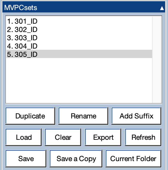
If you select all of the MVPCsets in the panel, you will see the decoding accuracy waveforms overlaid for each participant, as in the screenshot below.

To average across the five MVPCsets, go to the Average Across MVPCsets (Grand Average) panel. Make sure that it specifies all five MVPCsets (1:5) and that the option for computing the standard error is selected (as in the screenshot below).
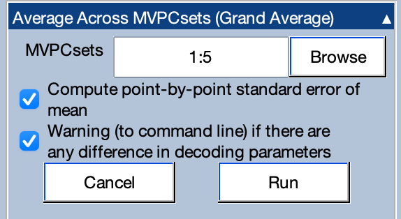
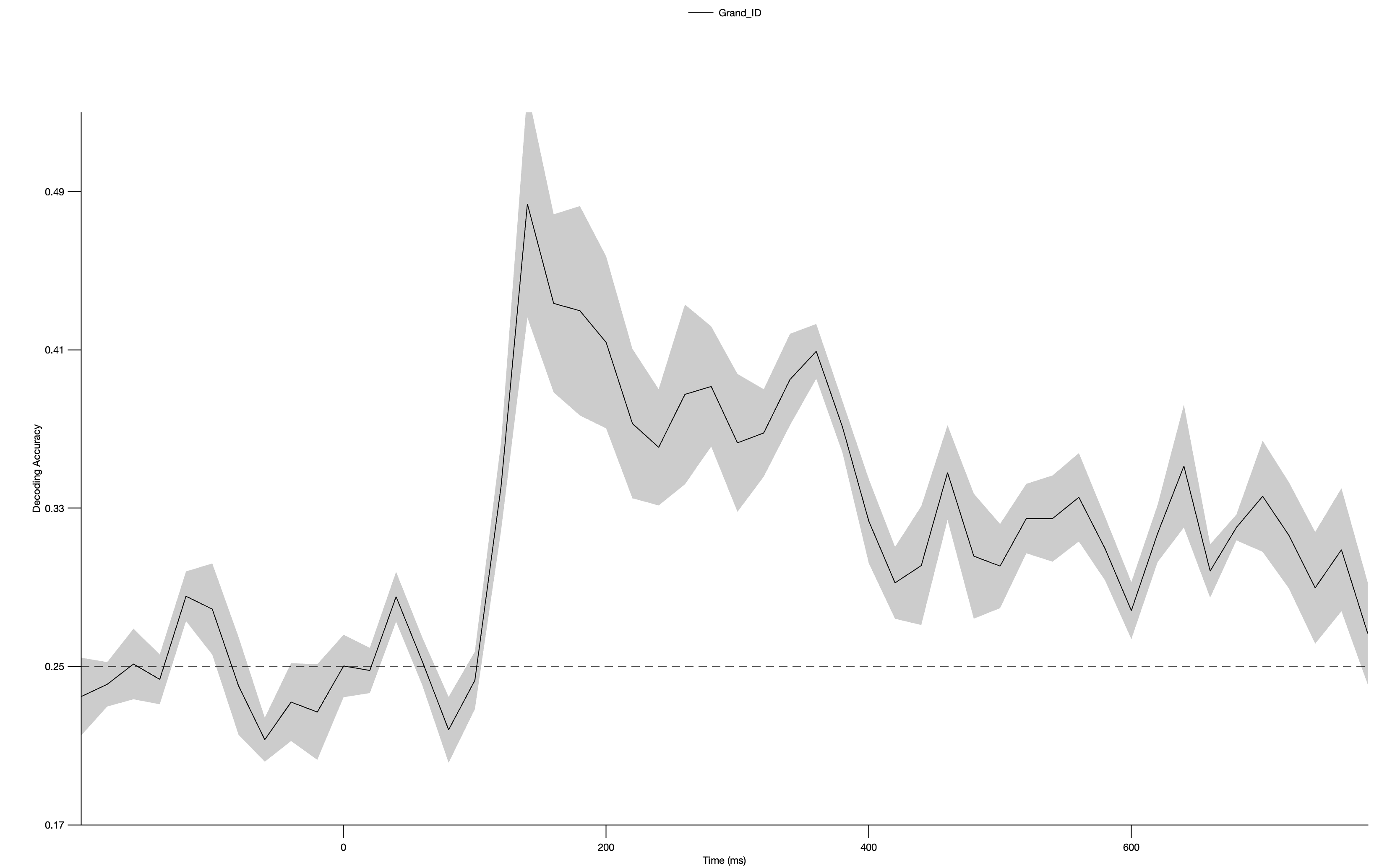
Click RUN. It will then ask you for the name of the new MVPCset, and you should use Grand_ID. You can save it to disk if desired. You will then see the resulting grand average decoding waveform as in the screenshot below.
Another useful exercise is to repeat all of these processes, but decoding the emotion expression rather than the face ID. To accomplish this, you just need to repeat the decoding step using classes 5–8 instead of classes 1–4. I recommend using Expression instead of ID in each of the MVPCset names. You can also find pre-made MVPCsets for emotion expression in the MVPCsets folder.
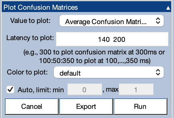
The confusion matrix at each time point is also saved in the MVPCset. This matrix gives you more information about the nature of the errors the decoder made. It’s easiest to explain this with an example. Make sure that Grand_ID is the active MVPCset, and then go to the Plot Confusion Matrices panel.
You can either plot a separate confusion matrix at each of several time points or have it average the matrices over a time range before plotting. Let’s do the second of these approaches by selecting Average Confusion Matrix between two latencies and entering 140 200 as the range of Latencies to plot (see the screenshot).
Click Plot and you will see something like the screenshot below.
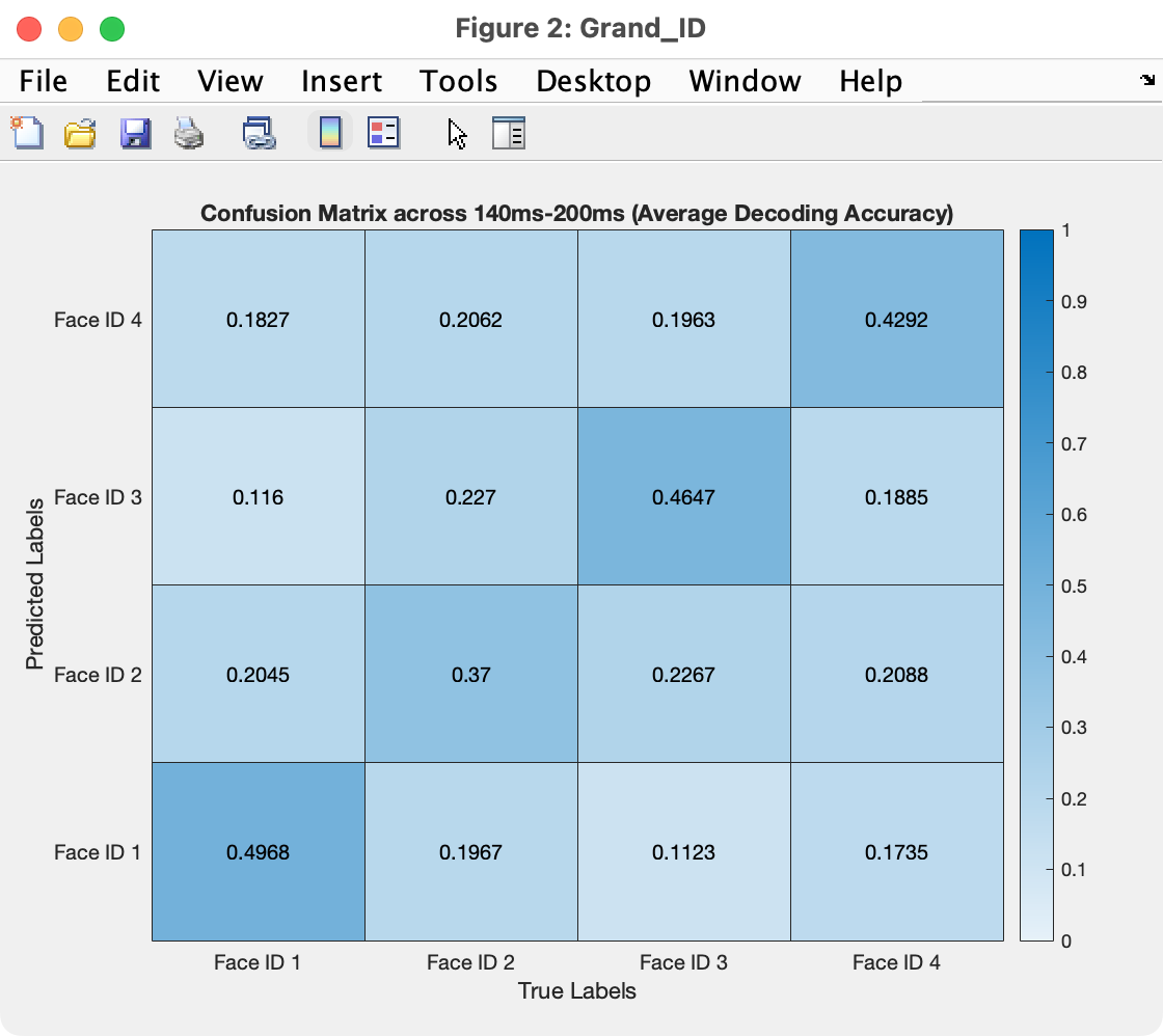
The figure shows a matrix of probabilities. The X axis is the set of true classes (ID 1, ID 2, ID 3, and ID 4), and the Y axis shows the class guessed by the decoder (also ID 1, ID 2, ID 3, and ID 4). The number in a given cell shows the probability that the decoder made the specified guess for the specified true class. This probability is also indicated by the coloring of the square.
The squares along the diagonal are the correct responses. You can see that face ID 2 was more difficult for the decoder to correctly guess (probability of 0.37) and face ID 1 was the easiest for the decoder to correctly guess (probability of 0.4968). In addition, when ID 1 was shown (i.e., when the true label was ID 1), the decoder was more likely to guess that it was ID 2 than ID 3.
You can export the confusion matrix values to a text file by clicking the Export button in the Plot Confusion Matrices panel. In addition, the matrix for each time point is stored in MVPC.confusions and can be accessed from scripts.