ATAC seq Data Processing
There are many ATAC-seq data processing pipelines available. For example:
Additionally, an interactive tutorial on how to process ATAC-seq data is available from the Galaxy Project Github page. All the methods mentioned use about the same approach for processing ATAC-seq, but do not include all the steps to generate an ATAC-seq signal track that is normalized for maxATAC.
This walkthrough details the steps that are necessary for retrieving and processing ATAC-seq data for use with maxATAC.
The overall workflow is implemented in several ways:
- The
maxatac preparefunction to process BAM files to min-max normalized bigwigs. - snakeATAC, a snakemake pipeline for ATAC-seq to process data from SRA.
- A common workflow language pipeline for ATAC-seq.
- A simple shell script.
The ATAC-seq experiments used for training maxATAC models are generated using the Illumina paired-end library format. The Illumina PE technology allows the sequencing of both DNA strands enabling placement of reads more accurately. This approach uses the same amount of DNA, but sequence both ends of the DNA fragment. PE sequencing is currently the standard for ATAC-seq and is the data type that this write-up focuses on.
ATAC-seq data analysis benefits from PE sequencing because open regions of chromatin can fall in repetitive regions or regions with structural variations. Using SE reads would increase the total sequencing depth required to achieve the same coverage as PE sequencing. One major contributor to this problem is that SE reads (35-100 bp) are harder to place with modern aligners, especially in regions containing repetitive and structural variants (Figure 1). PE sequencing helps in these cases by providing information about fragment size that can help alignment algorithms more accurately place the reads.
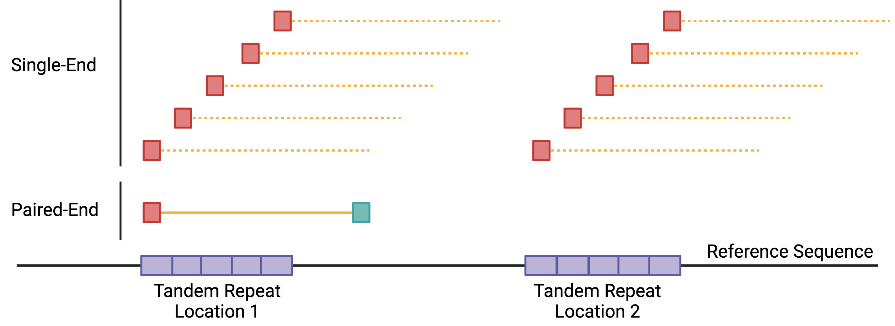
Additionally, PE data provides us information about sequencing fragment size distributions that can be used to infer nucleosome positioning[@Buenrostro2013]. The method for performing this type of analysis is covered later in assess fragment length distribution
Millions of next generation experiments have been performed across the world and deposited in public databases for free use by other scientists. Often, you will find yourself wanting to retrieve experimental data that might have been performed by another group to compare or supplement your own work. The quick access to sequencing data for use across the world is a hallmark of the National Center for Biotechnology Information (NCBI) databases such the short read archive (SRA) and gene expression omnibus (GEO) [@Wheeler2008].
GEO is a database that catalogues experimental data such as sequencing data, data analysis, and expression data related to the study of gene expression grouped by project[@Wheeler2008]. The GEO database helps organize sequencing data into coherent experiments and projects that are labeled by an accession that starts with the prefix GSM or GSE.
Most GEO entries will link to an entry in the SRA database of raw sequencing data that was used in the experiments. We use the GEO database to identify the raw sequencing data in the form of a .sra file that are stored in the SRA database.
The .sra files represent the raw data associated with a SRR ID record. We consider these to be technical replicates. The SRX ID is used to organize the may SRR IDs that can be associated with an experiment. We consider the SRX ID the biological replicate.
In addition to GEO, we will use data from the Encyclopedia of DNA Elements (ENCODE) [@Abascal2020] to supplement annotations available from GEO. The ENCODE data are QC'd, annotated, and reproducibility processed compared to data randomly generated and dumped in GEO. There is also overlap between the two databases, but sometimes there is a lag in deposits and annotations.
In this section, we will:
- Identify a maxATAC ATAC-seq sample that we are interested in.
- We will then use GEO and ENCODE to find the publicly available OMNI ATAC-seq raw data for download.
- Finally, we will download the sequencing data in
.sraformat from the SRA database and convert the reads to a.fastqfile. A.srafile is an archival format of next generation sequencing data used by NCBI to store the output of sequencing machines.
We have curated the cell types with ATAC-seq and ChIP-seq (as of July 2021) from multiple databases and this data is available in supplementary table 1 of the maxATAC publication. Additionally, the file maxATAC_v1_meta.tsv is an updated table is available with SRR IDs instead of ENCODE IDs.
For this example we will use MCF-7 from ENCODE as an example. The experimental meta information is available in the table below.
| ENCODE_ACCESSION | CELL_TYPE | ENCODE_BIO_REP | TECH_REP | BIO_REP | SOURCE |
|---|---|---|---|---|---|
| ENCSR422SUG | MCF-7 | 1 | SRR14103347 | SRX10475183 | ENCODE |
| ENCSR422SUG | MCF-7 | 2 | SRR14103348 | SRX10475184 | ENCODE |
The next few steps are geared towards using curated data from the maxATAC publication to find and download raw .fastq files. You can still use the following approaches for your own experimental data as well, you will just need to find the accession in your publication of interest.
If you want to skip downloading, alignment, and filtering, you can download the processed data from the maxATAC Zenodo page. The signal tracks are available for biological replicates.
This section focuses on downloading the samples that were derived from ENCODE.
The BIO_REP column in the maxATAC metadata corresponds to the individual experimental biological replicate. ENCODE samples in our meta data are labeled by the experiment accession. For example, the entry ENCSR422SUG_1 corresponds to the experiment ENCSR422SUG.
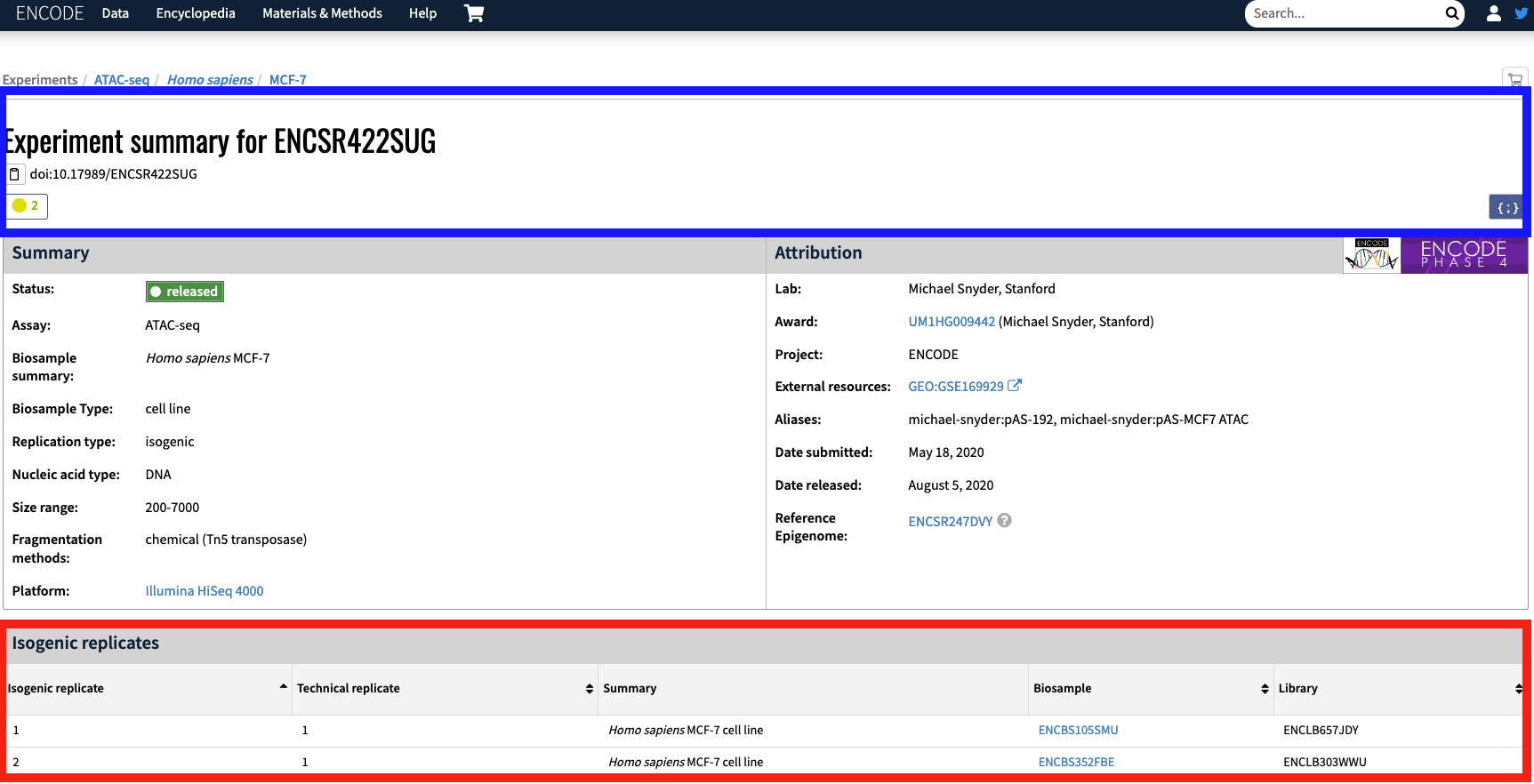
NOTE: The accession IDs found in the maxATAC metatable have the suffix _1 or _2 next to the ENCODE experimental ID to denote that we consider those entries to be biological replicates. The ENCODE definition of biological replicate is described below:
Biological replication – Replication on two distinct biosamples on which the same experimental protocol was performed. For example, on different growths, two different knockdowns, etc.
Isogenic replication – Biological replication. Two replicates from biosamples derived from the same human donor or model organism strain. These biosamples have been treated separately (i.e. two growths, two separate knockdowns, or two different excisions).
Technical replication – Two replicates from the same biosample, treated identically for each replicate (e.g. same growth, same knockdown).
The maxATAC metadata breaks the single ENCODE bioreplicate into two bioreplicates based on the available isogenic replicates (Figure 2; red box). For example, with experiment ENCSR422SUG, the isogenic replicate ENCBS105SMU corresponds to ENCSR422SUG_1.
You can download the ENCODE data by adding it to your ENCODE cart. The cart for all maxATAC data used from ENCODE is here. The cart allows you to build a meta file that can be used to systematically download the fastq files. The meta file for all ATAC-seq data used by maxATAC is here.
The easiest way to download these files is to use curl.
Example to download all ATAC-seq data:
xargs -L 1 -P 8 curl -O -J -L < ENCODE_ATAC_fastq.txtThe original ENCODE data curated by maxATAC was referencing ENCODE IDs. The updated maxATAC meta data for the ATAC-seq data references the individual SRR and SRX IDs. Therefore, this previous method is unnecessary.
Download .sra files and convert them to .fastq files with SRA prefetch and fasterq-dump using SRR ID
NCBI has developed a toolkit, SRAtoolkit, for interacting with genomics data in their databases. This toolkit has commands like prefetch and fastq-dump that can be used to retrieve publicly available sequencing data. The prefetch to fastq-dump workflow allows for pre-downloading SRA files and converting those files locally as needed.
Steps for downloading .sra files with SRAtoolkit:
- We use SRA
prefetchto pre-download the SRA file to our system. - Then we use
fasterq-dumpto convert the SRA file to.fastqformat.
The input to the prefetch function is the SRR or SRX ID.
> prefetch SRR14103347

2022-07-26T16:36:20 prefetch.2.10.1: 1) Downloading 'SRR14103347'...
2022-07-26T16:36:20 prefetch.2.10.1:  Downloading via https...
2022-07-26T16:44:13 prefetch.2.10.1:  https download succeed
2022-07-26T16:44:13 prefetch.2.10.1: 1) 'SRR14103347' was downloaded successfully
2022-07-26T16:44:13 prefetch.2.10.1: 'SRR14103347' has 0 unresolved dependenciesYou do not need to prefetch the .sra file before using fasterq-dump, but prefetching helps pre-download files for faster dumping. You can change the -e flag to fit the number of cores available.
> fasterq-dump -e 2 SRR14103347
spots read      : 45,575,539
reads read      : 91,151,078
reads written : 91,151,078The fasterq-dump function does not gzip files as they are converted to .fastq. This results in pretty large plain-text .fastq files. For example, the .fastq files for SRR14103347 total 24GB.
> du -h SRR14103347_*.fastq
 12G	SRR14103347_1.fastq
 12G	SRR14103347_2.fastq
If you gzip the files you can decrease the .fastq file size by more than half.
> pigz *.fastq
> du -h SRR14103347_*.fastq.gz
2.4G	SRR14103347_1.fastq.gz
2.6G	SRR14103347_2.fastq.gz
Most software can work with the gzipped files directly. This saves space and time. You should work with the gzipped files whenever possible and only unzip them as needed. Some .fastq files can be >30GB when unzipped.
If you are downloading a lot of SRA files and have limited space, make sure to use vdb-config -i to set the download path to a disk with enough space.
Technical replicates are concatenated into a single file per read. For all maxATAC samples, the biological replicate is the SRX ID and the technical replicates correspond to the SRR IDs.
The following code assumes that the technical replicates are in the same directory grouped by sample.
# cat read 1 technical replicates
> cat *_1.fastq.gz > ${srx}_1.fastq.gz

# cat read 2 technical replicates
> cat *_2.fastq.gz > ${srx}_2.fastq.gzAfter technical replicates are combined into a single biological replicate .fastq file, the reads can be QC'd. Quality control of reads is extremely important to generating high quality ATAC-seq signal tracks.
Reads produced from sequencing experiments use adapters to help index, prime, and keep track of reads in an experiment. These sequencing primers need to be removed before downstream data analysis.
The adapters contain the sequencing primer binding sites, the index sequences, and the sites that allow library fragments to attach to the flow cell lawn. Libraries prepared with Illumina library prep kits require adapter trimming only on the 3’ ends of reads, because adapter sequences are not found on the 5’ ends. Most of our experiments use paired-end Illumina sequencing technology, so we must process the .fastq file that is downloaded with that adapter trimming algorithm.
The steps for quality control of paired-end .fastq files:
- The read quality is assessed with
FastQC. - Adapter contamination and low quality bases are trimmed from reads.
- Assess read quality post trimming.
We use FastQC to assess the quality of the individual reads in each of the .fastq files. With ATAC-seq data, we are primarily interested:
- The overall quality of the reads in the file based on PHRED[@Ewing01031998] score
- The degree of sequence duplication
- The degree of adapter contamination
- The length of the reads
We will also use FastQC to assess read quality after adapter trimming. A wonderful guide to FastQC is available through the HBC Training Github page. In this section I will not describe all the statistics, but will focus on assessing the quality of the example sample we have been using.
The command for fastqc is simple. The -t 8 flag is used to set how many threads are available. Then the user provides a list of .fastq files. These files can be gzipped. Below is an example command and output.
> fastqc -t 8 *gz

Started analysis of SRR14103347_1.fastq.gz
Started analysis of SRR14103347_2.fastq.gz
Approx 5% complete for SRR14103347_1.fastq.gz
Approx 5% complete for SRR14103347_2.fastq.gz

...

Approx 95% complete for SRR14103347_1.fastq.gz
Approx 95% complete for SRR14103347_2.fastq.gz
Analysis complete for SRR14103347_1.fastq.gz
Analysis complete for SRR14103347_2.fastq.gz
The output of FastQC is a .html file and a .zip file with the data used in the analysis. The statistics from the .html file for SRR14103347_1.fastq.gz are shown in the examples below.
The PHRED score describes the quality of the base call from the sequencing machine. This value corresponds to:
Where Q is the PHRED score and P is the base-calling error probability.
| Phred Quality Score | Probability of incorrect base call | Base call accuracy |
|---|---|---|
| 10 | 1 in 10 | 90% |
| 20 | 1 in 100 | 99% |
| 30 | 1 in 1000 | 99.9% |
| 40 | 1 in 10,000 | 99.99% |
| 50 | 1 in 100,000 | 99.999% |
| 60 | 1 in 1,000,000 | 99.9999% |
Most reads used for ATAC-seq are greater than 75 bp long so triming low quality bases from the ends will not effect the mappability as much as say a 35 bp read. If you are using ChIP-seq data the PHRED score should be lower, at around 20.
The top of the FastQC output shows overall read statistics for the .fastq files.
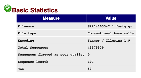
Important information in this section include the total sequences in the .fastq, the lengths of the reads, and the %GC content of the reads.
The field Sequences flagged as poor quality indicates that this .fastq file does not have any concerning sequences that are "low quality", but the reads could need additional processing as noted in the next sections.
The per base sequence quality score plot shows the distribution of PHRED scores at each base in the read. In the next step of read processing, adapter trimming, we will remove low quality base calls from the end of the read. We use a cutoff of PHRED >= 30.
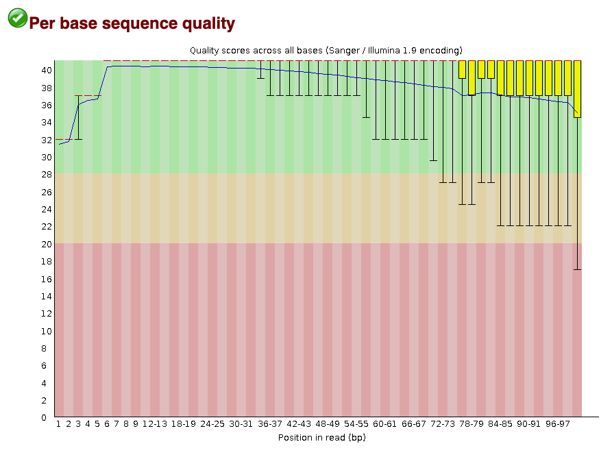
This plot shows that if you line all the reads up, the high quality base calls are found at the start of the read (Figure 5;bases 0-34). They gradually fall off as you travel down the read, with many dropping below the 30 cutoff. This is normal for sequencing experiments, but the majority of bases should be above your desired quality threshold.
The per sequence quality score metric shows the distribution of the mean PHRED score across all reads. That means for every read, the mean PHRED score was found. Then the distribution of those mean PHRED score for all of the reads in the .fastq were plotted.
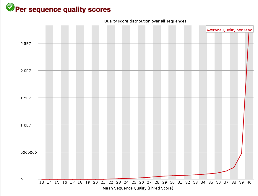
This plot shows that most reads have a mean PHRED score >37. This distribution is an example of high-quality reads in the .fastq. This mainly shows that the base-calling was accurate.
The per base sequence content plot shows the nucleotide composition at each base pair in the read. Each nucleotide is represented by a different colored line.
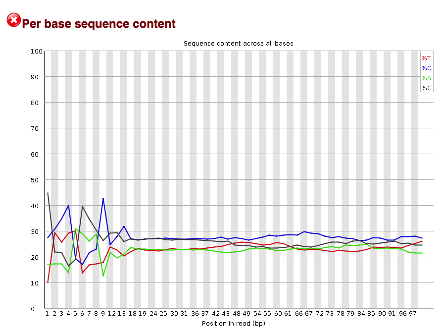
From this plot you can see there are nucleotide preferences at the 5' end of the read (left). This is common in ATAC-seq expriments due to the known Tn5 sequence bias. In other types of experiments, you would want a random distribution of nucleotides in the read. That is why this metric was originally flagged by FastQC.
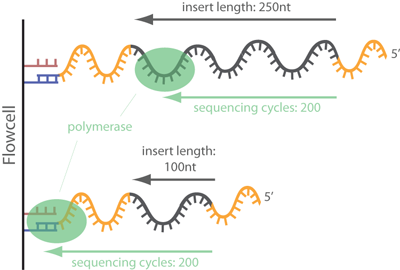
The next step is to identify any adapter contamination. If the insert size is less than the sequencing length, then the adapters at the 3' end of the read are included in the sequence. This excerpt from ecSeq Bioinformatics helps explain how adapters contaminate reads:
In common short read sequencing, the DNA insert (original molecule to be sequenced) is downstream from the read primer, meaning that the 5' adapters will not appear in the sequenced read. But, if the fragment is shorter than the number of bases sequenced, one will sequence into the 3' adapter. To make it clear: In Illumina sequencing, adapter sequences will only occur at the 3' end of the read and only if the DNA insert is shorter than the number of sequencing cycles (see picture below)!
The FastQC software will do a quick check to look for common adapters in a sample of the reads.
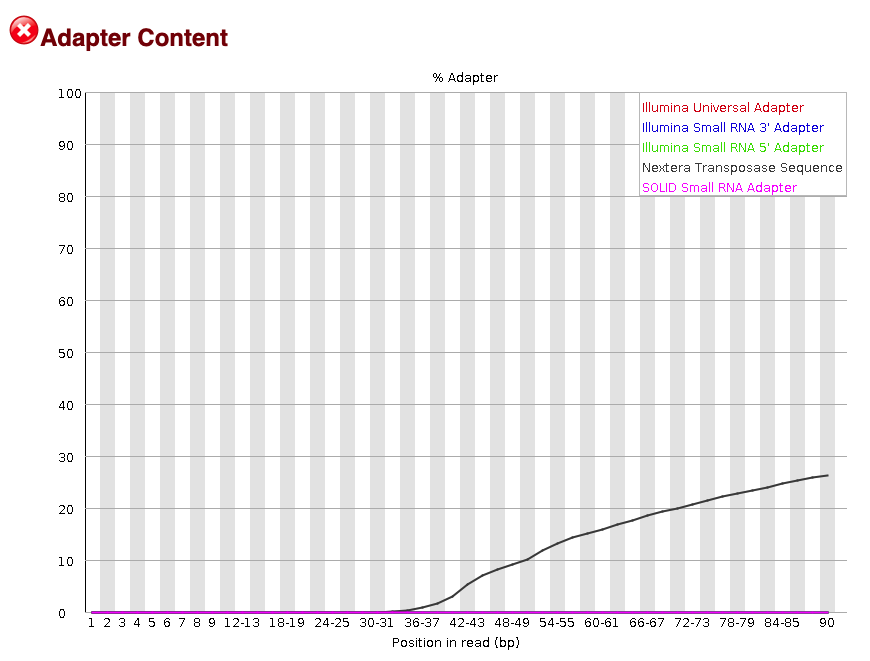
The adapter content plot shows adapter contamination from Nextera transposase sequences (Figure 8; black line). These adapters will be trimmed from the read to help increase mappability. Note that most adapter contamination occurs at the 3' end of the read, at mostly >36 bps.
The final metric that is important to look at is the level of sequence duplication across the reads. This metric looks at how much each read is duplicated.
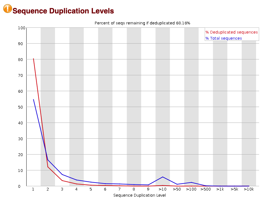
Our sample has a warning that the sequence duplication levels are a bit high. About 30% of the reads are duplicates. These could be caused by biological causes such as falling within repeat elements and also due to technical biases such as PCR duplication. We will account for duplication during our PCR deduplication step described later on.
We use Trim Galore! to trim adapters and low quality bases from the 3' ends of reads. Trim Galore! uses the popular Cutadapt algorithm with FastQC to apply adapter trimming.
We use the following command to trim adapters from reads:
> trim_galore -q 30 -paired -j 4 SRR14103347_1.fastq.gz SRR14103347_2.fastq.gzThe -q flag keeps only reads with a PHRED score 30 or greater.
The -paired flag is used to specify that the data is from paired-end sequencing experiments.
The -j 4 flag is used to specify that the jobs uses 4 threads, but at least 16 cores are needed. See documentation.
The next sections break up the output and provide a brief overview of the process used by Trim Galore!.
All of the parameters for the environment and run are listed on startup of Trim Galore!. The program will test for different version of cutadapt, whether pigz is installed, and what adapters are detected from sampling the reads.
Path to Cutadapt set as: 'cutadapt' (default)
Cutadapt seems to be working fine (tested command 'cutadapt --version')
Cutadapt version: 1.18
Could not detect version of Python used by Cutadapt from the first line of Cutadapt (but found this: >>>#!/bin/sh<<<)
Letting the (modified) Cutadapt deal with the Python version instead
pigz 2.6
Parallel gzip (pigz) detected. Proceeding with multicore (de)compression using 4 cores

No quality encoding type selected. Assuming that the data provided uses Sanger encoded Phred scores (default)Trim Galore! will start with auto-detecting adapters using a subsample of the reads. Any matches are reported.
AUTO-DETECTING ADAPTER TYPE
===========================
Attempting to auto-detect adapter type from the first 1 million sequences of the first file (>> SRR14103347_1.fastq.gz <<)

Found perfect matches for the following adapter sequences:
Adapter type	Count	Sequence	Sequences analysed	Percentage
Nextera	271028	CTGTCTCTTATA	1000000	27.10
smallRNA	0	TGGAATTCTCGG	1000000	0.00
Illumina	0	AGATCGGAAGAGC	1000000	0.00
Using Nextera adapter for trimming (count: 271028). Second best hit was smallRNA (count: 0)

Writing report to 'SRR14103347_1.fastq.gz_trimming_report.txt'
Trim Galore! detected Nextera adapters in 27% of the reads sampled with no other major contamination detected.
After adapters have been identified, use cutadapt to trim adapters from reads for the detected sequence:
SUMMARISING RUN PARAMETERS
==========================
Input filename: SRR14103347_1.fastq.gz
Trimming mode: paired-end
Trim Galore version: 0.6.7
Cutadapt version: 1.18
Python version: could not detect
Number of cores used for trimming: 4
Quality Phred score cutoff: 30
Quality encoding type selected: ASCII+33
Adapter sequence: 'CTGTCTCTTATA' (Nextera Transposase sequence; auto-detected)
Maximum trimming error rate: 0.1 (default)
Minimum required adapter overlap (stringency): 1 bp
Minimum required sequence length for both reads before a sequence pair gets removed: 20 bp
Output file(s) will be GZIP compressed

Cutadapt seems to be reasonably up-to-date. Setting -j 4
Writing final adapter and quality trimmed output to SRR14103347_1_trimmed.fq.gzThis next step shows the results from trimming the reads for bases with PHRED <30 and removing adapter contamination. The sequence CTGTCTCTTATA is searched for in all of the 3' ends of the sequencing reads.
  >>> Now performing quality (cutoff '-q 30') and adapter trimming in a single pass for the adapter sequence: 'CTGTCTCTTATA' from file SRR14103347_1.fastq.gz <<<
10000000 sequences processed
20000000 sequences processed
30000000 sequences processed
40000000 sequences processed
This is cutadapt 1.18 with Python 3.7.12
Command line parameters: -j 4 -e 0.1 -q 30 -O 1 -a CTGTCTCTTATA SRR14103347_1.fastq.gz
Processing reads on 4 cores in single-end mode ...
Finished in 285.77 s (6 us/read; 9.57 M reads/minute).

=== Summary ===

Total reads processed:              45,575,539
Reads with adapters:                25,001,500 (54.9%)
Reads written (passing filters):    45,575,539 (100.0%)

Total basepairs processed: 4,603,129,439 bp
Quality-trimmed:             230,108,812 bp (5.0%)
Total written (filtered):  3,854,541,276 bp (83.7%)

=== Adapter 1 ===

Sequence: CTGTCTCTTATA; Type: regular 3'; Length: 12; Trimmed: 25001500 times.

No. of allowed errors:
0-9 bp: 0; 10-12 bp: 1

Bases preceding removed adapters:
  A: 13.5%
  C: 40.6%
  G: 27.0%
  T: 18.8%
  none/other: 0.0%

Overview of removed sequences
length	count	expect	max.err	error counts
1	9194054	11393884.8	0	9194054
2	2148639	2848471.2	0	2148639
3	946834	712117.8	0	946834

...

100	106	2.7	1	5 101
101	91	2.7	1	37 54
The above statistics show that about 54% of reads have adapters detected. There are also statistics on the number of base pairs that have been quality trimmed. The total reads written decreases because some of the reads are discarded if >30% of the read sequence is ambiguous.
The same statistics are generated for read2, but only the summary results are shown for brevity.
=== Summary ===

Total reads processed:              45,575,539
Reads with adapters:                24,609,548 (54.0%)
Reads written (passing filters):    45,575,539 (100.0%)

Total basepairs processed: 4,603,129,439 bp
Quality-trimmed:             420,442,643 bp (9.1%)
Total written (filtered):  3,662,980,126 bp (79.6%)

=== Adapter 1 ===

Sequence: CTGTCTCTTATA; Type: regular 3'; Length: 12; Trimmed: 24609548 times.At the end of the process read pairs are validated for size according to the Trim Galore! manual. According to the manual:
This step removes entire read pairs if at least one of the two sequences became shorter than a certain threshold.
>>>>> Now validing the length of the 2 paired-end infiles: SRR14103347_1_trimmed.fq.gz and SRR14103347_2_trimmed.fq.gz <<<<<
Writing validated paired-end Read 1 reads to SRR14103347_1_val_1.fq.gz
Writing validated paired-end Read 2 reads to SRR14103347_2_val_2.fq.gz

Total number of sequences analysed: 45575539

Number of sequence pairs removed because at least one read was shorter than the length cutoff (20 bp): 1879987 (4.12%)

Deleting both intermediate output files SRR14103347_1_trimmed.fq.gz and SRR14103347_2_trimmed.fq.gz

====================================================================================================
The output of Trim Galore! that will be aligned to the genome will have the extension _{read}_val_{read}_.fq.gz like the file SRR14103347_1_val_1.fq.gz.
Reads are aligned to the reference genome using bowtie2[@Langmead2012]. We have tested other alignment algorithms (bwa-mem[@Li2009] and STAR[@Dobin2013]), but performance was similar across methods for maxATAC predictions.
After read alignment, the resulting alignments need to be quality controlled and explored with summary statistics such as fragment size distribution.
Additionally, low quality alignments, reads mapping to unwanted chromosomes, and PCR duplicates are excluded.
The metric we used to gauge the quality of read alignment is called the MAPQ score. This guide is usefule for understanding why we use MAPQ score.
| Flag | Description |
|---|---|
| 1 | read is mapped |
| 2 | read is mapped as part of a pair |
| 4 | read is unmapped |
| 8 | mate is unmapped |
| 16 | read reverse strand |
| 32 | mate reverse strand |
| 64 | first in pair |
| 128 | second in pair |
| 256 | not primary alignment |
| 512 | read fails platform/vendor quality checks |
| 1024 | read is PCR or optical duplicate |
We use the following command for aligning reads to the hg38 reference genome, make sure to use the output from Trim Galore!. The bowtie2 function can take some time to align your reads depending on the number of threads available and the size of the library. Therefore, bowtie2 alignment isn't included in the maxATAC package, but is included in snakeATAC and our shell scripts.
After generating a .bam file using the code below, you can use the maxatac prepare function to perform the filtering and signal generation.
> bowtie2 --very-sensitive --maxins 2000 -p 16 -x ./hg38/bowtie2_index/hg38 -1 SRR14103347_1_val_1.fq.gz -2 SRR14103347_2_val_2.fq.gz -S SRX10475183.samThe --very-sensitive setting defines a set of preset parameters for the matching algorithm that prioritize accuracy over speed.
The --maxins 2000 flag defines that maximum fragment size to 2,000 bp.
The -1 and -2 flags correspond to the .fastq files for reads 1 and 2, respectively.
The -S flag creates a .sam file as the output. This might not be the most effective use of hard disk space. Instead you can also use -b to output a .bam file. The trade-off is the speed and time required to compress the data.
The output from bowtie2 are simple summary statistics about alignment rate, number of discordant reads, and number of multi-mapped reads.
> bowtie2 --very-sensitive --maxins 2000 -p 16 -x ./hg38/bowtie2_index/hg38 -1 SRR14103347_1_val_1.fq.gz -2 SRR14103347_2_val_2.fq.gz -S SRR14103347.sam
43695552 reads; of these:
  43695552 (100.00%) were paired; of these:
    1391108 (3.18%) aligned concordantly 0 times
    36099610 (82.62%) aligned concordantly exactly 1 time
    6204834 (14.20%) aligned concordantly >1 times
    ----
    1391108 pairs aligned concordantly 0 times; of these:
      38497 (2.77%) aligned discordantly 1 time
    ----
    1352611 pairs aligned 0 times concordantly or discordantly; of these:
      2705222 mates make up the pairs; of these:
        2307127 (85.28%) aligned 0 times
        282955 (10.46%) aligned exactly 1 time
        115140 (4.26%) aligned >1 times
97.36% overall alignment rate
Sample SRR14103347 had an overall alignment rate of 97.36%. This is a very high alignment rate. The number of reads that mapped to more than one location was 14.20%. Depending on the ATAC-seq protocol, the degree of duplication can have a large range. In general, aim for <30%.
After the reads has been aligned to the genome, the aligned reads are filtered. Filtering alignments is important in order to remove PCR duplication events. The maxatac prepare function will perform the following steps given an input .bam or scATAC-seq fragments file. We want to remove reads that are the product of PCR duplicates. These are reads that have the exact same mapping position and barcode. This helps reduce the library specific bias caused by PCR amplification of random sequences.
We remove PCR duplicates using samtools sort to sort and then samtools fixmate to fix named read pairs. We then use samtools markdup to remove the duplicated reads. Some protocols use picard tools and this approach is also acceptable.
The first step will be to filter the reads by their MAPQ score and thensort the reads by name. We want to filter out low quality alignments before generating any signal tracks. To do this, we use the -q 30 flag with samtools view.
# Sort by NAME http://www.htslib.org/doc/samtools-sort.html
> samtools view -@ 8 -b -u -q 30 SRR14103347.bam | \
samtools sort -@ 8 -n -o SRR14103347_namesorted_q30.bam -After the reads are sorted by their names, samtools fixmate will fill in the information for their mates as stated in the documentation:
Fill in mate coordinates, ISIZE and mate related flags from a name-sorted or name-collated alignment.
# Fixmate and sort by POSITION then index http://www.htslib.org/doc/samtools-fixmate.html
> samtools fixmate -@ 8 -m SRR14103347_namesorted.bam - | \
samtools sort -@ 8 -o SRR14103347_fixmates.bam -

# The file needs to be indexed after sorting by position
> samtools index -@ 8 SRR14103347_fixmates.bamThe final step requires using samtools markdup to mark and remove duplicates. The output is position sorted and indexed.
# Mark duplicates, remove, sort, index
> samtools markdup -@ 8 -r -s SRR14103347_fixmates.bam - | \
samtools sort -@ 8 -o SRR14103347_deduplicated.bam -

> samtools index SRR14103347_deduplicated.bam
The -r flag with samtools markdup is used to remove the duplicates from the file.
The -s flag with samtools markdup prints some summary statistics shown below.
READ 87391104 WRITTEN 70733337
EXCLUDED 2307127 EXAMINED 85083977
PAIRED 84760956 SINGLE 323021
DULPICATE PAIR 16467008 DUPLICATE SINGLE 190759
DUPLICATE TOTAL 16657767
Out of 87391104 reads, 70733337 were written to output. In total there were 16657767 PCR duplicates.
Removing specific chromosomes while keeping only properly paired and oriented reads without singletons
The mitochondrial genome is abundant in every cell and in Standard ATAC-seq experiments there is a lot of mitochondrial contamination. We remove all reads associated with the mitochondrial genome from our analysis. Additionally, we focus on the autosomal chromsomes that are found in the reference genome.
During the filtering process we also want to double check that no singleton reads are stored in the BAM file. We use samtools to do perform filtering using the -f flag for inclusion of reads and the -F flag for exclusions of reads. We specify the -f 3 flag to filter for properly paired and oriented reads. We also want to make sure that the BAM file does not contain any unmapped reads either, so we use the samtools view flag -F 4 flag to exclude them.
We want to remove reads that are unmapped and singletons because we will use bedtools bamtobed to generate bed files for all entries. The pre-filtering ensures you only have the paired reads left when you convert your reads to a BED file, as each bed interval will be considered a cut-site in later processing.
This is an example:
> samtools view -@ 16 -f 3 -b -F 4 SRR14103347_deduplicated.bam chr1 chr2 chr3 chr4 chr5 chr6 chr7 chr8 chr9 chr10 chr11 chr12 chr13 chr14 chr15 chr16 chr17 chr18 chr19 chr20 chr21 chr22 chrX chrY | \
samtools sort -@ 16 -o SRR14103347_final.bam -
After the .bam file has filtered, we will next convert the read entries to BED intervals that represent the read as Tn5 cut sites.
The underlying enzyme that enables ATAC-seq is the Tn5 transposase. We want to leverage our knowledge of Tn5 biology and enzyme action to better resolve the exact location that the DNA was cut. We will generate cutsites using bedtools bamtobed, bedtools slop, and awk. For a more detailed description of Tn5 action during ATAC-seq, check out the original ATAC-seq publication from Jason Buenrostro[@Buenrostro2013], the HINT-ATAC paper, and the publication describing Tn5 for high-throughput sequencing.
The key steps to generating the ATAC-seq signal track are:
- Shift reads +4 bp on the (+) strand and -5 bp on the (-) strand.
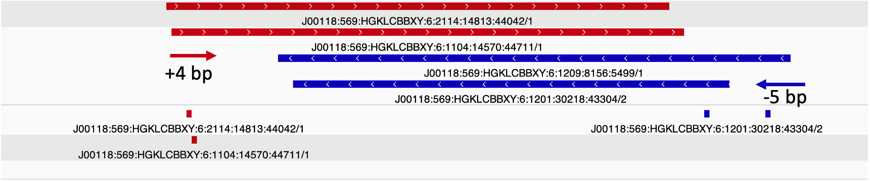
- Slop cut sites to 40 bp to smooth the sparse cut site signal. Image adapted from
HINT-ATAC.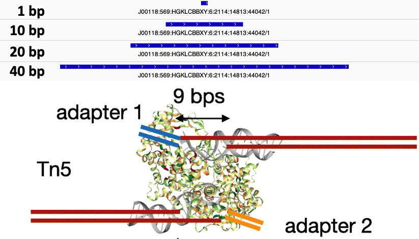
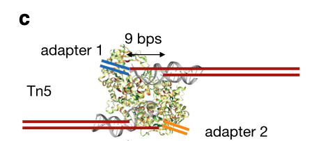
The Tn5 transposase homodimer cuts DNA to insert sequencing adapters. During transposition, two single stranded DNA ends are left at the 5' end that are 9bp long. The figure below is adapted from the HINT-ATAC publication and shows the crystal structure of Tn5 compared to the DNA it is bound to (Figure 8). Tn5 action causes two single strand 5' ends that are 9 bp long that are ligated to adapters.
Due to the 9 bp overhang, the read end does not correspond to the Tn5 cut site location. The true cut site location is located at the +5 bp position from the read end (Figure 9).
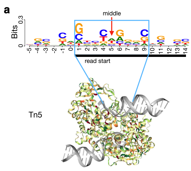
Identifying the exact cut site of the Tn5 enzyme allows for inferring the position of the enzyme and its cleavage point. To find the true cut site, the reads are shifted + 4 bp on the (+) strand and a -5 bp on the (-) strand.
We will convert our reads in the format of a .bam file to a .bed file where each read corresponds to a row in the file. This method will result in both ends of the paired end fragments being considered during signal generation. We use bedtools bamtobed to perform this conversion.
Example command:
bedtools bamtobed -i SRR14103347_final.bam > SRR14103347_reads.bedThis is an example of the output from converting the .bam to .bed:
> head SRR14103347_reads.bed
chr1	9989	10087	SRR14103347.10889469/1	0	+
chr1	9989	10083	SRR14103347.30379212/1	6	+
chr1	9990	10057	SRR14103347.15135894/1	0	+
chr1	9991	10090	SRR14103347.11934073/1	2	+
chr1	9996	10047	SRR14103347.10094158/1	6	+
chr1	9996	10095	SRR14103347.18169633/1	0	+
chr1	9996	10095	SRR14103347.25344866/1	1	+
chr1	9996	10047	SRR14103347.41806681/2	2	+
chr1	9997	10098	SRR14103347.22439821/2	2	+
chr1	9997	10098	SRR14103347.31445403/1	1	+
These .bed files can be large as they are not compressed and are plain text. If you are keeping these files you should gzip them.
In BED intervals the 5' of the (+) strand is found as the chromosome start position (column 2) and the (-) strand is found as the chromosome end position (column 3).
Once the reads are in .bed format, shifting the reads is easy with awk. In addition to shifting the reads. We only care about the position of the cut site, so we create a 1 bp window around the start 5' of the BED interval.
Example:
> awk 'BEGIN {OFS = "\t"} ; {if ($6 == "+") print $1, $2 + 4, $2 + 5, $4, $5, $6; else print $1, $3 - 5, $3 - 4, $4, $5, $6}' SRR14103347_reads.bed > SRR14103347_reads_shifted.bedThis is an example of shifted reads:
> head SRR14103347_reads_shifted.bed
chr1	9993	9994	SRR14103347.10889469/1	0	+
chr1	9993	9994	SRR14103347.30379212/1	6	+
chr1	9994	9995	SRR14103347.15135894/1	0	+
chr1	9995	9996	SRR14103347.11934073/1	2	+
chr1	10000	10001	SRR14103347.10094158/1	6	+
chr1	10000	10001	SRR14103347.18169633/1	0	+
chr1	10000	10001	SRR14103347.25344866/1	1	+
chr1	10000	10001	SRR14103347.41806681/2	2	+
chr1	10001	10002	SRR14103347.22439821/2	2	+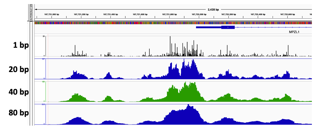
chr1 10001 10002 SRR14103347.31445403/1 1 +The final step is to center the signal over the 5' end of the read that represents the Tn5 transposase binding event. This will provide us with regions of the genome that are occupied by Tn5 which requires a minimal ~40bp accessible region to cleave DNA (figure 10).
)
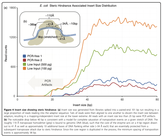
The window around the Tn5 cut size also helps to smooth the sparse cut site signal (figure 11).
Example code:
> bedtools slop -i SRR14103347_reads_shifted.bed.gz \
-g hg38.chrom.sizes \
-b 20 > SRR14103347_Tn5_slop20.bed
This is an example of reads with a -b 20:
> head SRR14103347_Tn5_slop20.bed
chr1	9973	10014	SRR14103347.10889469/1	0	+
chr1	9973	10014	SRR14103347.30379212/1	6	+
chr1	9974	10015	SRR14103347.15135894/1	0	+
chr1	9975	10016	SRR14103347.11934073/1	2	+
chr1	9980	10021	SRR14103347.10094158/1	6	+
chr1	9980	10021	SRR14103347.18169633/1	0	+
chr1	9980	10021	SRR14103347.25344866/1	1	+
chr1	9980	10021	SRR14103347.41806681/2	2	+
chr1	9981	10022	SRR14103347.22439821/2	2	+
chr1 9981 10022 SRR14103347.31445403/1 1 +There are many lists of exclusion regions available online. The list we curated for maxATAC was developed for ATAC-seq data specifically. Below is a list of blacklists that have been curated for maxATAC and their coverage statistics of the hg38 genome. The importance of removing these blacklist regions is further explored in the importance of data normalization.
| file | Number of Intervals | Total bps covered | Percent hg38 covered |
|---|---|---|---|
| ENCFF356LFX.bed | 910 | 71,570,285 | 2.17 |
| hg38-blacklist.v2.bed | 636 | 227,162,400 | 6.886 |
| hg38_centromeres.bed | 109 | 59,546,786 | 1.805 |
| hg38_gaps.bed | 827 | 161,348,343 | 4.891 |
| hg38_maxatac_blacklist.bed | 376 | 217,585,970 | 6.596 |
| hg38_maxatac_blacklist_V2.bed | 1,667 | 275,198,132 | 8.342 |
| hg38_segmental_dups_chrM.bed | 12 | 36,418 | 0.001 |
Example code:
> bedtools intersect -a SRR14103347_Tn5_slop20.bed -b /data/miraldiLab/databank/genome_inf/hg38/hg38_maxatac_blacklist_V2.bed -v > SRR14103347_Tn5_slop20_blacklisted.bedThis example had 1,952,443 of 66,223,862 Tn5 sites overlapping blacklist regions.
> wc -l SRR14103347_Tn5_slop20_blacklisted.bed
64271419 SRR14103347_Tn5_slop20_blacklisted.bed

> wc -l SRR14103347_Tn5_slop20.bed
66223862 SRR14103347_Tn5_slop20.bedThe above commands can be strung together into a single bash pipe for maximum efficiency!
> bedtools bamtobed -i SRR14103347.bam | \
awk 'BEGIN {OFS = "\t"} ; {if ($6 == "+") print $1, $2 + 4, $2 + 4, $4, $5, $6; else print $1, $3 - 5, $3 - 5, $4, $5, $6}' | \
bedtools slop -i - -g hg38.chrom.sizes -b 20 | \
bedtools intersect -a - -b hg38_maxatac_blacklist_V2.bed -v | \
sort -k 1,1 > SRR14103347_Tn5_slop20_blacklisted.bedThe final steps in processing your ATAC-seq data is to generate genome-wide signal tracks in .bigwig format that represent Tn5 counts at single-nucleotide resolution.
The overall steps are:
- Convert Tn5 sites in
.bedformat to.bedgraphformat where each position is a count of Tn5 intervals at each genomic location. - Convert Tn5
.bedgraphto.bigwigthat is normalized by sequencing depth
The blacklisted Tn5 counts file is used as input to bedtools genomecov with the -bg and -scale flags.
The -bg flag will output the counts in bedgraph format where the 4th column in the file corresponds to the Tn5 count.
Briefly, .bedgraph files are like .bed files, but represent ranges of values.
For example:
> bedtools genomecov -i SRR14103347_Tn5_slop20_blacklisted.bed \
-g hg38.chrom.sizes \
-bg > SRR14103347_Tn5_slop20_blacklisted.bedgraph

> head SRR14103347_Tn5_slop20_blacklisted.bedgraph
chr1	792554	792595	1
chr1	792617	792658	1
chr1	792838	792879	1
chr1	792884	792966	1
chr1	792982	793023	1
chr1	793050	793075	1
chr1	793075	793091	2
chr1	793091	793116	1
chr1	793213	793220	1
chr1	793220	793243	2
The -scale flag will normalize the signal at each position. We want to normalize the count by the # of mapped reads.
The below sections walk through how to calculate the scale factor for the -scale flag.
You can get the number of mapped reads from the .bam file used as input to the bedtools bamtobed function. The -c flag counts the reads. The -F 260 flag is used to exclude unmapped and non-primary alignments.
> mapped_reads=$(samtools view -c -F 260 SRR14103347_final.bam)
> echo $mapped_reads
66223862The scale factor is equal to each count divided by the mapped reads. Since bedtools genomecov -scale uses multiplication to apply to each value, we find the scale factor where,
> reads_factor=$(bc -l <<< "1/${mapped_reads}")
> echo $reads_factor
.00000001510029723123
Scale each value by 20,000,000. This is a value that was chosen for the maxATAC publication based ont he median sequencing depth of data available in 2021.
> rpm_factor=$(bc -l <<< "${reads_factor} * 20000000")
> echo ${rpm_factor}
.30200594462460000000
We use the value .30200594462460000000 for bedtools genomecov -bg -scale.
The final output should be a scaled count in .bedgraph format. These files must be sorted by position before being used with downstream software.
Example code:
> bedtools genomecov -i SRR14103347_Tn5_slop20_blacklisted.bed \
-g hg38.chrom.sizes \
-bg \
-scale .30200594462460000000 | \
LC_COLLATE=C sort -k1,1 -k2,2n > SRR14103347_Tn5_slop20_blacklisted_RP20M.bedgraph
Expected output:
> head SRR14103347_Tn5_slop20_blacklisted_RP20M.bedgraph
chr1	792554	792595	0.302006
chr1	792617	792658	0.302006
chr1	792838	792879	0.302006
chr1	792884	792966	0.302006
chr1	792982	793023	0.302006
chr1	793050	793075	0.302006
chr1	793075	793091	0.604012
chr1	793091	793116	0.302006
chr1	793213	793220	0.302006
chr1 793220 793243 0.604012Bigwig files are compressed wiggle files. These files represent spans of values that can be quickly accessed and visualized. We work primarily with the .bigwig signal tracks when using maxatac. We use a tool provided by UCSC called bedGraphToBigWig.
The following code uses the read-depth normalized .bedgraph file of Tn5 count as input:
bedGraphToBigWig SRR14103347_Tn5_slop20_blacklisted_RP20M.bedgraph hg38.chrom.sizes SRR14103347_Tn5_slop20_blacklisted_RP20M.bwThis represents the same information in the .bedgraph file, but in a more compressed and disk friendly format.
> du -h SRR14103347_Tn5_slop20_blacklisted_RP20M.bedgraph
2.2G	SRR14103347_Tn5_slop20_blacklisted_RP20M.bedgraph

> du -h SRR14103347_Tn5_slop20_blacklisted_RP20M.bw
472M SRR14103347_Tn5_slop20_blacklisted_RP20M.bwThis is an example workflow for read normalizing your inferred Tn5 bed files. This code will take the inferred Tn5 sites and build the genome wide coverage track using information in the bam header:
#!/bin/bash

########### RPM_normalize_Tn5_counts.sh ###########
# This script will take a BAM file and a BED file of insertion sites to create a bigwig file.

# This script requires that bedtools be installed and bedGraphToBigWig from UCSC

# INPUT1: BAM
# INPUT2: chromosome sizes file (hg38.chromsizes.txt)
# INPUT3: Millions factor (1000000 or 20000000)
# INPUT4: Name
# INPUT5: BED of Tn5 Sites

# OUTPUT: Sequencing depth normalized bigwig file scaled by # of reads of interest

# Set up Names
bedgraph=${4}.bg
bigwig=${4}.bw

mapped_reads=$(samtools view -c -F 260 ${1})
reads_factor=$(bc -l <<< "1/${mapped_reads}")
rpm_factor=$(bc -l <<< "${reads_factor} * ${3}")
echo "Scale factor: " ${rpm_factor}

# Use bedtools to obtain genome coverage
echo "Using Bedtools to convert BAM to bedgraph"
bedtools genomecov -i ${5} -g ${2} -bg -scale ${rpm_factor} | LC_COLLATE=C sort -k1,1 -k2,2n > ${bedgraph}

# Use bedGraphToBigWig to convert bedgraph to bigwig
echo "Using bedGraphToBigWig to convert bedgraph to bigwig"
bedGraphToBigWig ${bedgraph} ${2} ${bigwig}

rm ${bedgraph}If your experiments include multiple biological replicates for the same condition, you can average the normalized signal using maxatac average. The detailed instructions about using maxatac average are found on the average wiki page and readme.
Example command:
maxatac average --bigwigs SRX10474876_Tn5_slop20_blacklisted.bw SRX10474877_Tn5_slop20_blacklisted.bw --prefix IMR-90During the initial development of maxATAC in 2020, we based our method on Leopard[@Li2021] which is a method developed for Dnase signal tracks used in the 2017 ENCODE-DREAM challenge. Our experience with Leopard introduced us to the importance of many key concepts of deep learning in genomics. This section focuses on the importance of signal normalization.
We found that one key aspect of model performance was data normalization.
However, the quality of the reference sample can influence to the distribution of scores.
Our performance on these models was near 0, with many odd observations.
Detailed instruction about min-max normalization implemented by maxATAC is documented on the normalize wiki page and readme.
Example command:
maxatac normalize --signal GM12878_RP20M.bw --prefix GM12878 --output ./test --method min-max --max_percentile 99We use macs2 to identify regions of the genome that are enriched for signal compared to background, these regions are called "peaks" (islands, windows, hotspots). The peaks represent a binary label that is used to identify the enriched regions. Peak calling can be accomplished by many types of software, and the peaks themselves can be refined using additional downstream analysis. This is our approach for finding regions of the genome with high Tn5 cut site signal compared to background.
Depending on your experimental design, macs2 can be used with biological replicates as inputs in addition to a control group. We do not use a control input when calling peaks.
We will input the SRR14103347_Tn5_slop20_blacklisted.bed file. This bed file has been filtered, PCR deduplicated, converted to Tn5 cut sites, and had blacklisted regions removed.
The macs2 software has many parameters and settings that can be used to tune peak calling. We will take advantage of the --shift, --ext_size, and -bed input parameters.
Example command:
macs2 callpeaks -i -n --shift 0 --ext_size 40bamPEFragmentSize -b {input} -p {threads} --binSize {params.bin_size} --blackListFileName {params.blacklist} --outRawFragmentLengths {output}