Math AutomaticDifferentiation
A short introduction to the use of dual numbers and hyper-dual numbers in automatic differentiation can be found at https://en.wikipedia.org/wiki/Automatic_differentiation. for a more in-depth intro there are the papers of Jeffrey A. Fike in the internet. for the implementation (only the forward mode is implemented) i relied mainly on his paper http://enu.kz/repository/2011/AIAA-2011-886.pdf, where the first 10 pages are a relatively concise and straightforward explanation of these things.
Lets say we want to calc the first derivative at several points of this function:
f(x) = ex / ( sin(x)3 + cos(x)3 )1/2
Lets put that into a block:
f:=[:x|x exp / ((x sin raisedToInteger: 3) +(x cos raisedToInteger: 3))sqrt]. a dual number can consist of a value and its derivative. if we want to know the value of f' at x = 1.5 we construct a PMDualNumber this way, as the derivative of the identity function is 1:
anX:= PMDualNumber value: 1.5 eps:1.
f value:anX.
Hence f(1.5) is 4.497780053946163, lets check that:
f value:1.5."--> 4.497780053946163"
"and the value of f'(1.5) is 4.053427893898621"
just to check this result, it is:
f'(x) = ex( 3 cos(x) + 5 cos(3 x) + 9 sin(x) + sin(3 x)) / ( 8 ( sin(x)3 + cos(x)3 )3/2)
1.5 exp*(1.5 cos *3 +((3*1.5)cos *5)+(1.5 sin *9)+(3*1.5)sin)/
 ((((1.5 sin raisedToInteger: 3) + (1.5 cos raisedToInteger: 3))
 raisedTo: (3/2))*8).
"--> 4.053427893898622"
this result is not too different.
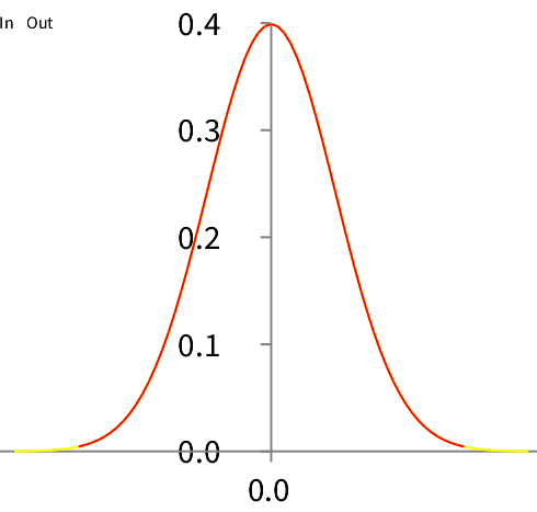
For the following visualization you'd need to have Roassal2 loaded which can be found at http://www.smalltalkhub.com/#!/~ObjectProfile/Roassal2. lets differentiate the error function (of Math-DHB-Numerical) and see whether we get the normal distribution. normally you can use the errorFunction like this:
3 errorFunction ."--> 0.9986500327777648"but since i have not implemented errorFunction for dual numbers (i guess its unnecessary), i've to use a trick, that is unproblematic since DhbErfApproximation has a unique instance:
g:=[:x| DhbErfApproximation new value: x].
h:=DhbNormalDistribution new.
b := RTGrapher new.
ds := RTDataSet new.
ds noDot.
ds points: (-4 to: 4 by:0.1).
ds y: [:i|h value:i].
ds x: #yourself.
ds connectColor: (Color yellow).
b add: ds.
b add: ds.
ds := RTDataSet new.
ds noDot.
"here ive to use another trick as #errorFunction has a singularity at 0
insofar as it always returns Float 0.5 instead of computing the result:"
ds points: ((-3 to: 3 by:0.1)collect:[:i|i=0 ifTrue:[1e-10]ifFalse:[i]]).
ds y: [:i|(g value:(DualNumber value: i eps: 1)) eps].
ds x: #yourself.
ds connectColor: (Color red).
b add: ds.
b build.
b view openWithMenu
the yellow normaldistribution curve is indeed nicely covered by the red derivative curve.
ok so far, while a DualNumber can be seen as a number that consists of a value and and its first derivative, a HyperDualNumber has in a way a value, two first (partial) derivatives and a second (partial) derivative. hence if you want to calc the second derivative of f at 1.5 you can do it this way:
f value:(HyperDualNumber value: 1.5 eps:1 eps2:1 eps1eps2:0) ."-->
 HyperDualNumber(value: 4.497780053946163 eps1: 4.053427893898621
                eps2: 4.053427893898621 eps12: 9.463073681596601)"
you see that f'' is 9.463073681596601 and the rest of the result is as the calc with a DualNumber. if you would calc f'' directly from the formula for f'' you would do this:
1.5 exp*(130 - ((2*1.5)cos * 12) + ((4*1.5) cos *30) +((6*1.5)cos *12)-
 ((2*1.5)sin *111)+((4*1.5) sin *48)+((6*1.5)sin *5))/(((
 (1.5 sin raisedToInteger: 3) + (1.5 cos raisedToInteger: 3))
 raisedTo: (5/2))*64)."--> 9.463073681596606"
hence the result is not too far off from the best possible result.
a more complicated way to calculate f'' would be to stack 2 DualNumbers into each other:
f value:(DualNumber value: (DualNumber value: 1.5 eps:1) eps:1)."-->
 DualNumber(value: DualNumber(value: 4.497780053946163 eps: 4.053427893898621)
 eps: DualNumber(value: 4.053427893898621 eps: 9.463073681596605))"
here we get f'' = 9.463073681596605. of course you can use that method to calc higher derivatives, for examples to calculate f''' you could stack a DualNumber into a HyperDualNumber or so.
you can see that in general you can use those numbers simply like you normally use numbers. you just have to take care of the few methods from Numbers, that are not implemented in DualNumbers and of non-differentiable points like in the graphic example above.
to see some further advantages & disadvantages lets implement newton's zero-finding method, that uses this refinement
xi+1 = xi - (f(xi) / f'(xi))
it is rather simple with DualNumbers (docu how to use Fixpoint can be found here):
fp:=Fixpoint new .
fp block:
	[:value| |f|
		f:=function value: value.  "function is as yet undefined"
		f eps ~=0 ifTrue:
			[value value: value value - (f value/f eps)].
		value eps: 1] .
lets find the next local zero near 1.0 of this function:
f(x) = x3 + 2 x2 + x
function := [:x|(x raisedToInteger: 3)+(2*x squared)+x].
fp value: (DualNumber value:1.0 eps:1).
fp evaluate."--> DualNumber(value: 0.0 eps: 1)"
fp iterations."--> 9"
the result x = 0.0 obviously is exact. now in DHB-Numerical there is DhbNewtonZeroFinder to do the same by using an approximation of the derivative. lets compare:
fp2 :=DhbNewtonZeroFinder new.
fp2 setFunction: function.
fp2 initialValue: 1.0.
fp2 desiredPrecision: 1e-20."with this fp2 uses 9 iterations as fp"
fp2 evaluate ."-->  4.3377098873975624e-33"
fp2 iterations."--> 9"
well, what would you expect with this desiredPrecision? but if you compare the speed DhbNewtonZeroFinder clearly wins:
fp verbose: false.
fp2 desiredPrecision: 1e-20.
[fp value: (DualNumber value:1.0 eps:1).fp evaluate]bench." '6,738 per second'"
[fp2 initialValue: 1.0.fp2 evaluate]bench ." '19,042 per second'"
this is generally so, derivative calculations via (hyper-)dual numbers are more exact as calculation via a simple approximation, but they are usually slower. a detailed explanation of this can be found eg in http://enu.kz/repository/2011/AIAA-2011-886.pdf.
an obvious advantage though is that they are simple to use. as another example lets implement a local extremum finder again using newton's method:
xi+1 = xi - (f'(xi) / f''(xi))
mf := Fixpoint new .
mf block:
	[:hyperDualValue| |d|
		d:=function value: hyperDualValue.
		d eps1eps2 ~=0 ifTrue:
			[d:=d eps/d eps1eps2.
			hyperDualValue value: hyperDualValue value - d].
		hyperDualValue eps: 1;eps2: 1;eps1eps2: 0] .
mf value:(HyperDualNumber value: 1.0 eps: 1 eps2: 1 eps1eps2: 0).
mf evaluate."-->
 HyperDualNumber(value: -0.33333333333333337 eps1: 1 eps2: 1 eps12: 0)"
function value: mf result."-->
 HyperDualNumber(value: -0.14814814814814814 eps1: 0.0 eps2: 0.0 eps12: 2.0)"
obviously -0.148148 is a minimum of f at x = -0.333333 since f'' = 2.0 is positive. lets have a look at the function:
b := RTGrapher new.
ds := RTDataSet new.
ds noDot.
ds points: (-1.7 to: 0.3 by:0.01).
ds y: [:i|function value:i].
ds x: #yourself.
ds connectColor: (Color red).
b add: ds.
b build.
b view openWithMenu .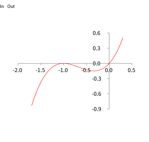
one can see that we should get a maximum if we start on the left side:
mf value:(HyperDualNumber value: -2.0 eps: 1 eps2: 1 eps1eps2: 0).
mf evaluate. "-->HyperDualNumber(value: -1.0 eps1: 1 eps2: 1 eps12: 0)"
function value: mf result."-->
 HyperDualNumber(value: 0.0 eps1: 0.0 eps2: 0.0 eps12: -2.0)"
the expected maximum with a negative f''.
lets turn to functions of several variables. like for example
f(x,y) = x y2 + x
if you want to know the gradient of f at the point x = 2, y = 2 you could do it like this:
f := [:i| |x y| x := i first. y := i second. x * y squared + x].
f value: (Array with: (DualNumber value: 2 eps:1) with: 2)."-->
 DualNumber(value: 10 eps: 5)"
f value: (Array with: 2 with: (DualNumber value: 2 eps:1))."-->
 DualNumber(value: 10 eps: 8)"
or you simply use Gradient:
g:=Gradient of:f.
g value:#(2 2) ."--> #(5 8)"
"or some other values:"
g value:#(1 3) ."--> #(10 6)"
another utility object is Hessian, which returns a DhbSymmetricMatrix:
h := Hessian of:f.
h value:#(2 2)."-->
a DhbVector(0 4)
a DhbVector(4 4)"
h value:#(1 3)."-->
a DhbVector(0 6)
a DhbVector(6 2)"
"Hessian also calcs as a byproduct the gradient:"
h gradient." #(10 6)"
if you want to see how to calculate a partial second derivative with HyperDualNumbers, you can simply look at the straightforward implementation of Hessian>>value: