Math KernelSmoothing
if you have some data and want to estimate its density without making assumptions about the form of the underlying distribution, iow if you want a non-parametric estimation you can use KernelSmoothedDensity. you could also use a histogram, but this has the drawback that the density of a histogram is not continuous and rough, a KernelSmoothedDensity is in a way a smoothed continuous histogram. let's make an example:
r := Random new.
data := (1 to: 1000) collect: [:each| r next]
of course we know that these data follow a uniform distribution and knowing this we could construct a very good density, lets do that first:
h := PMHistogram new.
data do:[:each| h accumulate: each].

hd:= PMHistogrammedDistribution histogram: h.
density:= PMUniformDistribution from: 0 to: 1."just for comparing purposes"

plt := RSChart new.
x := -0.24 to:1.24 count: 100.
p1 := RSLinePlot new x: x y: (x collect: [:each| hd value: each]).
plt addPlot: p1.

p2:= RSLinePlot new x:x y: (x collect: [:each| density value: each]).
plt addPlot: p2.

plt addDecoration: RSHorizontalTick new.
plt addDecoration: RSVerticalTick new.
plt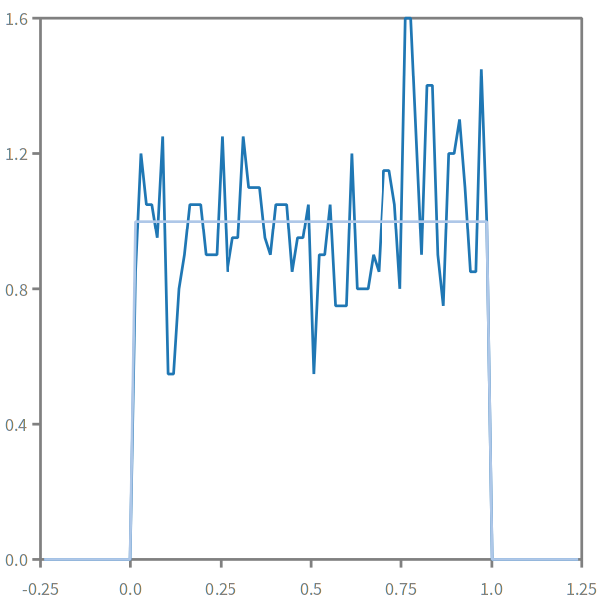
this density is very wiggly and its jumps can make it difficult to use. knowing that it follows a uniform distribution we can make of course this:
ud := PMUniformDistribution fromHistogram: h
"Uniform distribution( 0.002630064020919476, 1.0204437218750617)"
a distribution which conforms very well with variabledensity which obviously is "Uniform distribution( 0, 1)".
btw this method to estimate a distribution via fromHistogram: is a rather general one implemented for most PMProbabilityDensities, it just estimates the distribution parameters from the histogram parameters, hence it is fast and simple but it does not necessarily work as fine as it works for uniform distributions. in more complicated cases there are PMLeastSquareFit and PMMaximumLikelihoodHistogramFit (see the Dhb-book), or for special fitting procedures one can also use FunctionFit. I have not implemented KernelSmoothedDensity>>fromHistogram: because, if one has a PMHistogram one usually also has the original data, and the result is more exact with the original data, although calculation via a histogram would be faster; perhaps i should also implement fromHistogram: for big-sized data, since then calculation via the data will be slow, much slower than the calculation via binned data from the histogram.
after this short digression let us proceed with PMKernelSmoothedDensity. since we know that the underlying density is not continuous, it theoretically does not make sense to make a continuous PMKernelSmoothedDensity out of it, but i think it is instructive to see how PMKernelSmoothedDensity deals with the discontinuities of the distribution at 0 and 1.
hence let us now assume we know nothing about the underlying distribution, and lets continue with this nonsense-example and see what we get, when we make a PMKernelSmoothedDensity out of these data:
k := PMKernelSmoothedDensity fromData: data.
"KernelSmoothedDistribution (dataSize: 1000 kernel: 'normal' bandWidth: 0.06642325603894135)"
with this we can do almost everything, that we can do with a ProbabilityDensity:
k average.
"0.5015623721208247"
data average.
"0.5015623721208246"
"they are the same, well, occasionally there are tiny rounding errors"

k standardDeviation.
"0.29036725454021733"
data stdev.
"0.28322009331774073"
"the standardDeviation of a KernelSmoothedDensity is always a little bit
higher than the standardDeviation of the underlying data"
Lets have a look at the density:
plt := RSChart new.
x := -0.24 to:1.24 count: 100.
p1 := RSLinePlot new x: x y: (x collect: [:each| k value: each]).
plt addPlot: p1.

p2:= RSLinePlot new x:x y: (x collect: [:each| density value: each]).
plt addPlot: p2.

plt addDecoration: RSHorizontalTick new.
plt addDecoration: RSVerticalTick new.
plt
or the cdf:
b := RTGrapher new.
ds := RTDataSet new.
ds noDot.
ds points: (-0.24 to: 1.24 by:0.02).
ds y: [:i|k distributionValue: i].
ds connectColor: (Color blue).
b add: ds.
ds := RTDataSet new.
ds noDot.
ds points: (-0.24 to: 1.24 by:0.02).
ds y: [:i|density distributionValue: i].
ds connectColor: (Color gray).
b add: ds.
b build.
b view openWithMenu . 
there are 2 settable parameters in PMKernelSmoothedDensity: the kernel and the bandwidth.
the kernel defines the smoothing method and can be set via:
-
kernel:which expects a block with a function, whose integral is 1 and for which f(x)=f(-x) -
normalwhich sets the kernel to the normal distribution (this is the default) -
epanechnikovobviously the epanechnikov kernel.
usually different kernels dont make much difference in the result, hence normally you dont need to change the default. but lets see what the difference is in our example:
k1:=k copy.
k1 epanechnikov .
k1."-->
KernelSmoothedDistribution (dataSize: 1000 kernel: 'epanechnikov'
                            bandWidth: 0.06597473318785621)"
b := RTGrapher new.
ds := RTDataSet new.
ds noDot.
ds points: (-0.24 to: 1.24 by:0.02).
ds y: [:i|k value: i].
ds connectColor: (Color blue).
b add: ds.
ds := RTDataSet new.
ds noDot.
ds points: (-0.24 to: 1.24 by:0.02).
ds y: [:i|k1 value: i].
ds connectColor: (Color red).
b add: ds.
b build.
b view openWithMenu . 
you see, the kernel doesn't really matter. but if you inspect the red curve carefully you'll see a few sharp bends in it, iow although the density calculated via epanechnikov is continuous, it is not differentiable everywhere. (the reason is that the epanechnikov kernel itself is not differentiable everywhere.)
the bandwidth defines the smoothing intensity. it can be read with bandWidth and written by bandWidth: or ruleOfThumbBandWidth. by default Silverman's rule of thumb is used, which normally works quite well and if you want to change the bandwidth you can use the default number as a starting point. let's see, how changing the bandwidth, changes the result.
k bandWidth ."--> 0.06597473318785621"
k1:=k copy.
k1 bandWidth: 0.09.
k2:=k copy.
k2 bandWidth: 0.045.
k2."-->
KernelSmoothedDistribution (dataSize: 1000 kernel: 'normal' bandWidth: 0.045)"
b := RTGrapher new.
ds := RTDataSet new.
ds noDot.
ds points: (-0.24 to: 1.24 by:0.02).
ds y: [:i|k value: i].
ds connectColor: (Color blue).
b add: ds.
ds := RTDataSet new.
ds noDot.
ds points: (-0.24 to: 1.24 by:0.02).
ds y: [:i|k1 value: i].
ds connectColor: (Color red).
b add: ds.
ds := RTDataSet new.
ds noDot.
ds points: (-0.24 to: 1.24 by:0.02).
ds y: [:i|k2 value: i].
ds connectColor: (Color green).
b add: ds.
ds := RTDataSet new.
ds noDot.
ds points: (-0.24 to: 1.24 by:0.002).
ds y: [:i|density value: i].
ds connectColor: (Color black).
b add: ds.
b build.
b view openWithMenu . 
i'd say, the blue default bandwidth is actually quite good. well, this is what you get if you smooth a discontinuous density with such big jumps as a uniform density.