Quick start to ODE

The following code shows how to obtain the numerical solution of a simple one-dimensional ODE. Note the configuration of the stepper type showing the flexibility of the library. We solve the simple ODE x' = 3/(2t^2) + x/(2t) with initial condition x(1) = 0 and step size 0.1.

|dt system stepper solver| 
dt := 0.1. 
system := PMExplicitSystem block: [:x :t | 3.0 / (2.0 * t * t) + (x / (2.0 * t))]. 
stepper := PMRungeKuttaStepper onSystem: system. 
solver := (PMExplicitSolver new) stepper: stepper; system: system; dt: dt. 
solver solve: system startState: 0 startTime: 1 endTime: 10

Every time, you need to solve an ODE, you will need to setup three different object: a system that represent an or a set of ODEs, a stepper that deals with the method that will be used to solve your ODE and finally a solver.

With the PMExplicitSystem block you can represent as a function of 2 arguments (t and x), the rhs (right hand side) of the differential equation: dx/dt = f(x,t).

Let's try to do plot the behavior of an compartimental model in epidemiology like SIR:

|solver state system dt beta gamma values stepper diag|
dt := 1.0.
beta := 0.01.
gamma := 0.1.
system := PMExplicitSystem block: [ :x :t| |c|
	 c := Array new: 3.
	 c at: 1 put: (beta negated) * (x at: 1) * (x at: 2).
	 c at: 2 put: (beta * (x at: 1) * (x at: 2)) - (gamma * (x at: 2)).
	 c at: 3 put: gamma * (x at: 2).
	 c
	 ].
stepper := PMRungeKuttaStepper onSystem: system.
solver := (PMExplicitSolver new) stepper: stepper; system: system; dt: dt.
state := #(99 1 0).
values := (0.0 to: 200.0 by: dt) collect: [ :t| state := stepper doStep: state 
                                                          time: t stepSize: dt ].

Using Graph-ET for visualising the infectious evolutionary diagram:

For only one diagram:

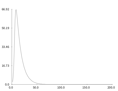
diag := GETDiagramBuilder new.
diag lineDiagram 
	models: (1 to: 200 by: 1);
	y: [ :x| (values at: x) at: 2 ];
	regularAxis.
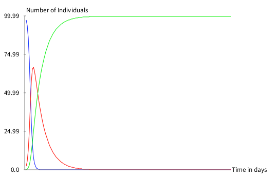
diag open.

For a composite diagram of S (blue), I (red) and R (green)

|colors|
diag := OrderedCollection new.
colors := Array with: Color blue with: Color red with: Color green.
1 to: 3 do: [ :i|
	diag add: 
		((GETLineDiagram new)
			models: (1 to: 200 by: 1);
			y: [ :x| (values at: x) at: i ];
			color: (colors at: i))
	 ].
builder := (GETDiagramBuilder new).
builder compositeDiagram 
	xAxisLabel: 'Time in days';
	yAxisLabel: 'Number of Individuals';
	regularAxis;
	diagrams: diag.
builder open.

Let's try to implement the Lorenz attractor as the a set of 3 differential equations, that we will solved with a Runge-Kutta solver:

| solver stepper system dt sigma r b state values diag|
sigma := 10.0.
r := 28.
b := 8.0/3.0.
dt := 0.01.
system := ExplicitSystem
block: [:x :t | | c |
   c:= Array new: 3.
   c at: 1 put: sigma * ((x at: 2) - (x at: 1)).
   c at: 2 put: r * (x at: 1) - (x at: 2) - ((x at: 1) * (x at: 3)).
   c at: 3 put: (b negated * (x at: 3) + ((x at: 1) * (x at: 2))).
   c].
stepper := RungeKuttaStepper onSystem: system.
solver := (ExplicitSolver new) stepper: stepper; system: system; dt: dt.
state := #(10.0 10.0 10.0).

values := (0.0 to: 100.0 by: dt) collect:[:t |
   state := stepper doStep: state time: t stepSize: dt.
   state].

We can try to visualize the result by using GraphET:

diag := GETDiagramBuilder new.
(diag scatterplot)
   models: values;
   x: [: v | v at: 1 ];
   y: [: v | v at: 2 ];
   regularAxis;
   dotSize: 1.
diag open

As there are different case what value to write for system, stepper and solver here you have a hint:

(Pay attentions: for first 3 methods you should write your order of method like thisAB3Stepper. )

Methods	System	Stepper	Solver	Comment
Adams - Bashforth method of order n=2,3,4	ExplicitSystem	ABnStepper	ABnSolver
Adams - Moulton method of order n=3,4	ImplicitSystem	AMnStepper	AMnSolver
Backward differentiation formulas method of order n=2,3,4	ImplicitSystem	BDFnStepper	BDFnSolver
Beckward Euler method	ImplicitSystem	ImplicitStepper	ImplicitSolver
Euler method	ExplicitSystem	ExplicitStepper	ExplicitSolver
Heun method	ExplicitSystem	HeunStepper	ExplicitSolver	Heun's method may refer to the improved or modified Euler's method (that is, the explicit trapezoidal rule), or a similar two-stage Runge-Kutta method.
Implicit midpoint method	ImplicitSystem	ImplicitMidpointStepper	ImplicitMidpointSolver
Midpoint method	ExplicitSystem	MidpointStepper	ExplicitSolver
Runge-Kutta method (order 4)	ExplicitSystem	RungeKuttaStepper	ExplicitSolver
Trapezoidal rule	ImplicitSystem	TrapezoidStepper	ImplicitSolver	It is Adams - Moulton method of order 2