Cell formatting using Format function

Format([Column], "format string")

You can use the Format function in column formulas to specify the formatting to apply to the columns. If you want all values in the column to use the same format string, you will typically just set the format string in the Column styles formatting pane.

However, if you want to apply different format strings to cells in a column based on which row they are on, you can use the Format() function in a column calculation to conditionally apply different format strings to the cells in the column.

Example
This example shows how to apply a custom format string to specific cells in a column using the Format function.
In particular, we want to apply a custom format string to the cells of the Sales and Accounts Receivables lines.

1. Go to Edit mode
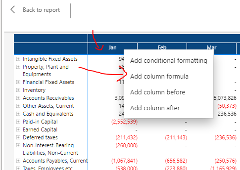
2. Right-click the column header that you want to apply custom formatting to, then choose "Add column formula"

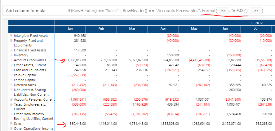
3. In the Formula editor, enter the following formula:
   IF(RowHeader() == "Sales" || RowHeader() == "Accounts Receivables", Format([Column], "#,#.00"), [Column])

You get the [Column] token ([Jan] in this example) into the formula at the current caret position by clicking a cell in the column.

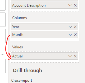
Note! In this example, the [Jan], [Feb], etc columns all come from the Actuals field in the Values bucket, so the rule will apply to all the Actuals columns (Jan, Feb, Mar, etc), not just Jan which we right clicked.