Soft Computing project, Software Engineering and Information Technologies, Undegraduate Academic Studies, Faculty of Technical Sciences, University of Novi Sad, 2019/2020
Technologies used: Keras 2.3.1, Python 3.6.1, Tensorflow 2.0.0
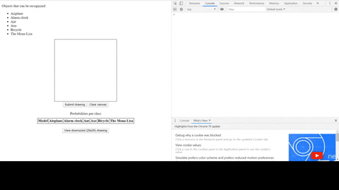
The goal is to predict what the user has drawn on the canvas. A subset of the „Quick, Draw!“ dataset was used, which included the following six classes: Airplane, Alarm clock, Ant, Axe, Bicycle, The Mona Lisa.
-
clone the project via
git clone https://github.com/UrosOgrizovic/SimpleGoogleQuickdraw.git -
download data (see Fetching the data)
-
in terminal, enter
set WRAPT_INSTALL_EXTENSIONS=false(this is required due to apip install tensorflowproblem) -
in terminal, enter
pip3 install -r requirements.txtto install the dependencies -
download VGG weights and place them in
models/transfer_learning: -
run
web.py
Create a folder called data in project root, download and place the following files into that folder:
Airplane: https://storage.cloud.google.com/quickdraw_dataset/full/numpy_bitmap/airplane.npy
Alarm clock: https://storage.cloud.google.com/quickdraw_dataset/full/numpy_bitmap/alarm%20clock.npy
Ant: https://storage.cloud.google.com/quickdraw_dataset/full/numpy_bitmap/ant.npy
Axe: https://storage.cloud.google.com/quickdraw_dataset/full/numpy_bitmap/axe.npy
Bicycle: https://storage.cloud.google.com/quickdraw_dataset/full/numpy_bitmap/bicycle.npy
The Mona Lisa: https://storage.cloud.google.com/quickdraw_dataset/full/numpy_bitmap/The%20Mona%20Lisa.npy
13 layers, excluding the input layer (view architecture visualization). Dropout was used to avoid overfitting. The kernel's dimensions are 3x3, which is an often-used kernel size.
This model was trained on both 10,000 images per label and 100,000 images per label. The latter case brought no noticeable improvement.
Callbacks used:
-
ImageDataGenerator was used for augmenting the images, which helps avoid overfitting.
-
EarlyStopping was especially useful for the 100k-images-per-label-model, as it greatly reduced the number of epochs that the model would execute before stopping. It was set up in such a way that if the validation loss was noticed to have stopped decreasing after five epochs, the training would terminate.
-
ModelCheckpoint was used with the
save_best_onlyflag set toTrue, so as to only save the latest best model (i.e. the best model out of all the epochs) according to the validation loss. -
ReduceLROnPlateau was used because models often benefit from reducing the learning rate by a factor of 2-10 once learning stagnates [2]. Yet again, the monitored value was the validation loss.
Constraints used:
- MaxNorm is a type of weight constraint. From Dropout: A Simple Way to Prevent Neural Networks from Overfitting: "One particular form of regularization was found to be especially useful for dropout—constraining the norm of the incoming weight vector at each hidden unit to be upper bounded by a fixed constant c."
Plots:
The default value of 1 was used for C, the penalty error term. 'rbf' was the value used for the kernel parameter, also by default. The default value of 'scale' was used for gamma, the RBF kernel coefficient.2
Training was very slow; from docs: "The fit time scales at least quadratically with the number of samples and may be impractical beyond tens of thousands of samples." This model doesn't work well on this problem.
A "grid search" on C and gamma was performed using cross-validation [1].
Perhaps the performance of this model could be improved by using the histogram of oriented gradients (HOG).
2C tells the SVM optimization how much to avoid misclassifying each training example by (large C - small hyperplane, and vice versa), and gamma defines how far the influence of a single training example (i.e. point) reaches (large gamma - the decision boundary will only depend on the points close to it - that is, each point's influence radius will be small, and vice versa).
Consists of 24 layers, excluding the input layer (view architecture visualization). However, instead of using VGG19's fully connected layers, I used my own, because my problem doesn't have 1000 classes. Additionally, I had to pad Google's 28x28 images to 32x32 images, because this model doesn't accept images smaller than 32x32.
This model uses 3x3 convolution filters. Its predecessor, VGG16, achieved state-of-the-art results in the ImageNet Challenge 2014 by adding more weight layers compared to previous models that had done well in that competition.
| set | CNN 10k | CNN 100k | SVM 2k | SVM 10k | VGG 10k | VGG 100k |
|---|---|---|---|---|---|---|
| train | ~99% | ~97% | ~89%* | ~84%* | ~94% | ~94% |
| validation | ~99% | ~97% | ~94% | ~94% | ||
| test | ~96% | ~98% | ~89%* | ~84%* | ~94% | ~94% |
* 10-fold cross validation was done for the SVM models, so there are only train and test accuracies