KPS is a free and open source, flexible, efficient software infrastructure for simultaneous orbital and attitude propagation of satellites in Low Earth Orbit (LEO), using real-time attitude-based analytical (frontal area-based) OR collision-based aerodynamics simulation, for Windows and Linux. Gravitational, magnetic, and atmospheric modeling is performed. Magnetic and gravity gradient torques are considered. Fast propagation at excellent accuracy is performed by a custom Adams-Bashforth-Moulton linear multistep numerical integrator written in C++.
Realtime visualization and other useful tools are dually available as MATLAB(r) (GNU Octave compatible) and Python utilities included with KPS. This project is designed for direct application by CubeSat teams and other groups interested in aerodynamic stabilization of satellites in Low Earth Orbit. It is also designed for education in itself as a comprehensive infrastructure that covers a wide range of topics fusing aerospace and performance computing.
KPS is licensed under the MIT License: https://opensource.org/licenses/mit-license.php
Copyright (c) 2017 Kareem Omar
Permission is hereby granted, free of charge, to any person obtaining a copy of this software and associated documentation files (the "Software"), to deal in the Software without restriction, including without limitation the rights to use, copy, modify, merge, publish, distribute, sublicense, and/or sell copies of the Software, and to permit persons to whom the Software is furnished to do so, subject to the following conditions:
The above copyright notice and this permission notice shall be included in all copies or substantial portions of the Software.
THE SOFTWARE IS PROVIDED "AS IS", WITHOUT WARRANTY OF ANY KIND, EXPRESS OR IMPLIED, INCLUDING BUT NOT LIMITED TO THE WARRANTIES OF MERCHANTABILITY, FITNESS FOR A PARTICULAR PURPOSE AND NONINFRINGEMENT. IN NO EVENT SHALL THE AUTHORS OR COPYRIGHT HOLDERS BE LIABLE FOR ANY CLAIM, DAMAGES OR OTHER LIABILITY, WHETHER IN AN ACTION OF CONTRACT, TORT OR OTHERWISE, ARISING FROM, OUT OF OR IN CONNECTION WITH THE SOFTWARE OR THE USE OR OTHER DEALINGS IN THE SOFTWARE.
KPS makes use of four external libraries:
-
GeographicLib: https://sourceforge.net/projects/geographiclib/files/distrib/ GeographicLib is also licensed under the MIT license.
-
glm: http://glm.g-truc.net/ glm is also licensed under the MIT license.
-
Clipper: http://www.angusj.com/delphi/clipper.php Clipper is licensed under the 2003 Boost Software License: http://www.boost.org/LICENSE_1_0.txt
-
Eigen: http://eigen.tuxfamily.org/ Eigen is licensed under the MPL2 license: https://www.mozilla.org/en-US/MPL/2.0/
Head to https://github.com/komrad36/KPS for the latest version! Feel free to contact me at kareem.omar@uah.edu with any questions.
No. I provide precompiled binaries for those who just want to use the application and not study its code or modify it. Furthermore, they are statically compiled, so you don't have to download any runtime libraries at all. The executables just work, standalone, on both Windows and Linux.
The Windows executable is called 'KPS.exe'. The Linux executable is called 'KPS'.
Here are instructions for Windows and Linux:
You'll need Microsoft Visual Studio 2015. Open 'KPS.sln' in Visual Studio.
Three external libraries are needed:
- GeographicLib: https://sourceforge.net/projects/geographiclib/files/distrib/
- glm: http://glm.g-truc.net/
- Eigen: http://eigen.tuxfamily.org/
Download Eigen and GLM (they’re header only!) and install GeographicLib. Point Visual Studio to them in the KPS project’s configuration, under Configuration Properties -> VC++ Directories. You’ll need to modify the Include Directories for all three, and the Library Directories just for GeographicLib.
My Include Directories and Library Directories look like this, respectively, for Release x64:
C:\glm;C:\Eigen;C:\GeographicLib-1.45_VS2015\include;$(VC_IncludePath);$(WindowsSDK_IncludePath);

C:\GeographicLib-1.45_VS2015\windows\Release64;$(LibraryPath)
Just modify the entries to match the include and lib locations where you installed the libraries.
The Visual Studio solution actually contains 7 projects – KPS itself and its 6 supporting projects. Those are all Python projects (also available in MATLAB/Octave) and don’t need compiling. You can just run them directly with Python 3.4.
Make sure KPS itself (the first project listed) is selected, and you’re ready to build.
Three external libraries are needed:
- GeographicLib: https://sourceforge.net/projects/geographiclib/files/distrib/
- glm: http://glm.g-truc.net/
- Eigen: http://eigen.tuxfamily.org/
Download Eigen and GLM (they’re header only!) and install GeographicLib. Open the ‘Makefile’ and adjust the Includes and Library paths if needed (you probably won’t have to if you let every library install to its default location).
NOTE: my Makefile compiles KPS with the AVX instruction set enabled for better performance. If your processor does not support AVX, edit the Makefile and remove all instances of the switch "-mavx".
The KPS main propagator is run with just one argument: a configuration file. This means, if your graphical environment supports it, that you can drag-and-drop a config file onto the KPS executable to start a run with that configuration.
The configuration file specifies 22 parameters required by KPS to operate, in any order. Blank lines are ignored. Comments can be entered by beginning a line with #. Capitalization is ignored. A sample configuration file looks like this:
POLY_FILE = poly.kps
MAG_GAIN = 25e3
TIME_SINCE_EPOCH_AT_DEPLOY = 0.0
GRAV_MODEL = wgs84
PROPAGATOR = abm
AERO_MODE = ANALYTICAL
ABS_TOL = 1e-6
REL_TOL = 2.3e-14
AERO_PITCH = 0.01
MAX_STEP_SIZE = 26000
MAG_MODEL = wmm2015
MAG_YEAR = 2016
BINARY_OUTPUT = true
REALTIME_OUTPUT = true
SAT_CM = 0, 0, 0
SAT_INIT_POS = 6871000, 0, 0
SAT_INIT_V = 0, 5385.72, 5385.72
SAT_INIT_Q = 1, 0, 0, 0
SAT_INIT_W = 0.008, -0.05, 0.003
SAT_MASS = 8.0
SAT_MOI = 0.0667, 0, 0, 0, 0.0867, 0, 0, 0, 0.0333
TIME_SPAN = 500000
These parameters will now be explained individually:
POLY_FILE = a relative or absolute path to a polygon file containing a list of vertices comprising quadrilaterals that define the satellite body. Typical value: poly.kps
MAG_GAIN = a positive magnetorque gain factor. Magnetorque is currently coded to react against the satellite’s angular velocity, attempting to slow down the satellite’s rotation. Specify a 0 gain factor to disable magnetic torque. Typical value for CubeSat: 30000
TIME_SINCE_EPOCH_AT_DEPLOY = seconds since epoch (when the ECI and ECEF frame coincide) at the start of simulation. Typical value: 0
GRAV_MODEL = the GeographicLib gravity model to use for gravitational acceleration. Higher quality models are slower. Available models are: "POINT", "WGS84", "EGM84", "EGM96", and "EGM2008". In order to use a model (other than POINT), you must download the (small) gravity model file for that model from http://geographiclib.sourceforge.net/html/gravity.html. Typical value: wgs84
PROPAGATOR = the numerical integrator to use. Available integrators are: “RKDP” and “ABM”. The first is a Runge-Kutta Dormand-Prince pair solver, like MATLAB’s ode45(). The second is a faster and more accurate Adams-Bashforth-Moulton linear multistep solver, like MATLAB’s ode113(). ABM should generally be used.
AERO_MODE = Specify ANALYTICAL to use area-based analytical aerodynamics force and torque computation. See the KPS research paper for more information. Specify GRID to use collision-based aerodynamics. ANALYTICAL is recommended as it is the most accurate, yet still quite fast. GRID with very coarse pitch settings is likely to be the absolute fastest option if extreme accuracy is not desired.
ABS_TOL = the absolute tolerance of the intergrator. Tighter (smaller) tolerances result in slower propagation. Typical value: 1e-6
REL_TOL = the relative tolerance of the intergrator. Tighter (smaller) tolerances result in slower propagation, but unlike absolute tolerance, a low relative tolerance is critical for a chaotic system like satellite propagation. Typical value: 2.3e-14
AERO_PITCH = if in collision-based (GRID) aerodynamics mode, this is the linear pitch between test particle collisions for the aerodynamics engine, in meters. This value is IGNORED if ANALYTICAL aero mode is in use. Smaller pitch results in more accurate aerodynamics, but simulation time increases with the inverse square of this value, so don’t make it too small! Choose a value accurate enough to nicely cover the satellite surface. For a CubeSat, 0.005 to 0.03 is a good starting point (i.e. between 5 mm and 3 cm from one simulated collision to the next). Typical value: 0.01
MAX_STEP_SIZE = the maximum step size in seconds between two steps during integration. The integrators are both adaptive step size, meaning that they adjust the step size as necessary to maintain the requested tolerances while moving as fast as they can. This value doesn’t usually need to be adjusted. Typical value: 26000
MAG_MODEL = the GeographicLib magnetic model to use for local Earth magnetic field determination (used for magnetic torque). Higher quality models are slower. Available models are: "WMM2010", "WMM2015", "IGRF11", "IGRF12", "EMM2010", and "EMM2015". In order to use a model, you must download the (small) magnetic model file for that model from http://geographiclib.sourceforge.net/html/magnetic.html. Typical value: wmm2015
MAG_YEAR = the year for which the magnetic model will return data. Earth’s magnetic field changes over time, so the GeographicLib models require the year as an input. Typical value: 2016
BINARY_OUTPUT = either ‘true’ or ‘false’. ‘true’ causes the outputs of KPS to be packed double-precision floating point values. This is the fastest option and is the ONLY one that works with KPS_Vis, the realtime and post visualization tool included with KPS. If, however, you want to be able to easily read and export the data, specify ‘false’ to produce ASCII .csv files instead. Typical value: ‘true’
REALTIME_OUTPUT = either ‘true’ or ‘false’. ‘true’ causes KPS to flush the output buffer after every write so KPS_Vis, the realtime visualization, can immediately and smoothly display the latest data. Disabling this option will not affect final output but may cause realtime visualization to look choppy or fail altogether, but may (slightly) increase performance. Typical value: ‘true’
SAT_CM = the center of mass of the satellite in the Body frame. Useful if you want to experiment with different CMs without having to shift all the coordinates in the polygon file, which is what would be required if I assumed the CM was always at the origin. Separate the three components x, y, and z by commas. For example - typical value: 0, 0, 0
SAT_INIT_POS = the satellite’s initial position in the ECI frame in meters. Separate the three components x, y, and z by commas. For example - typical value: 6871000, 0, 0
SAT_INIT_V = the satellite’s initial velocity in the ECI frame in meters per second. Separate the three components x, y, and z by commas. For example - typical value: 0, 5385, 5385
SAT_INIT_Q = the satellite’s initial orientation as a unit quaternion (a versor) representing a rotation of the ECI frame into the Body frame, or equivalently, a vector in the Body frame into the ECI frame. Separate the four components w, x, y, and z by commas. For example - typical value: 1, 0, 0, 0
SAT_INIT_W = the satellite’s initial angular velocity in the Body frame in radians per second. Separate the three components x, y, and z by commas. For example - typical value: 0.008, -0.05, 0.003
SAT_MASS = the mass of the satellite in kilograms. Typical value: 4
SAT_MOI = the moment of inertia matrix of the satellite. To simplify input, pass in the 9 elements separated by commas, moving along one row, then the next. In other words, if the matrix looks like this:
a b c
d e f
g h i
You would specify ‘a, b, c, d, e, f, g, h, i’ in the configuration file. Typical value: 0.0667, 0, 0, 0, 0.0867, 0, 0, 0, 0.0333
TIME_SPAN = the number of seconds to simulate. You can abort the simulation early at any time by closing the console window or pressing CTRL+C. Typical value: 500000
A sample configuration file, 'config.kps', is included.
The only other requirement to run KPS is the data for the magnetic and gravitational model specified in the configuration file, as mentioned above. Magnetic models are provided by GeographicLib in the form of a small download available here: http://geographiclib.sourceforge.net/html/magnetic.html#magneticinst
If the user specifies a gravity model of POINT, no download is needed. For a more complex model, the appropriate data can similarly be downloaded from here: http://geographiclib.sourceforge.net/html/gravity.html#gravityinst
To help users quickly generate different test orbits, I provide the KPS_GenOrbit tool (in both Python and MATLAB/Octave, as with all the ancillary tools around KPS). KPS_GenOrbit is the simplest of these utilities. It allows the user to turn a requested orbit, such as “500 x 600 km at 40° inclination”, into the SAT_INIT_R and SAT_INIT_V (initial position and velocity) parameters required by the configuration file.
For an x by y kilometer altitude elliptical orbit at i inclination (in degrees), simply call the utility like:
KPS_GenOrbit <x> <y> <i>
The satellite will begin at the x portion of the orbit. For example, a 500 x 600 km orbit at 40° inclination in which the satellite begins at 500 km is requested as follows:
KPS_GenOrbit 500 600 40
The system responds:
Generating stats for a 500x600 km orbit at 40°...
SAT_INIT_POS = 6871000, 0, 0
SAT_INIT_V = 0, 5855.6619518398, 4913.4837840876
That’s it! The bottom two lines can be copied and pasted directly into a KPS configuration file.
The polygon files expected by KPS specify the geometry of the satellite as a series of polygons. By default, these polygons must be quadrilaterals, although this can be changed if necessary (a recompile is required).
Up to 512 quadrilaterals are supported. Each quadrilateral consists of four coplanar points, each listed on its own line in the polygon file. Each point is a 3-vector in the Body frame with components in meters, separated by commas. The points must be in order, i.e. a line drawn from the first, through the second, through the third, through the fourth, and back to the first must complete the outline of the polygon. For example, a square with one corner at the origin, with area 1, lying entirely in the first quadrant of the x-y plane, could be defined by a portion of the polygon file that looks like this:
0, 0, 0
0, 1, 0
1, 1, 0
1, 0, 0
There are other valid representations; what matters is that the points “flow” either clockwise or counter-clockwise such that a line drawn through them in order (and back to the first point again) would outline the polygon and not cross itself.
After listing one polygon, simply list the next after it. Leaving a blank line is optional; they are ignored. List as many polygons as is required to define your satellite. The order of the polygons does not matter, only the order of the vertices within each polygon.
A sample polygon file, 'poly.kps', is included.
The KPS_GenPoly tool helps generate these files by allowing the user to customize a Python or MATLAB script to generate numerical values.
For example, consider a satellite whose geometry includes a solar panel that can deploy at different angles. Say the user wishes to run KPS on several different panel angles. Rather than having to manually compute the numerical values of the solar panel polygon for every deployment angle, the user can enter an expression such as 0.5+cos(panel_angle) in the KPS_GenPoly script.
The entire polygon can be constructed this way, in terms of variables chosen freely by the user. These variables can then be set at the top of the script, and the script can then be executed to output a polygon file with the correct numerical values. Changing the panel angle, in this case, would simply require changing the variable at the top and re-running the script, and KPS would be ready to simulate the new angle immediately.
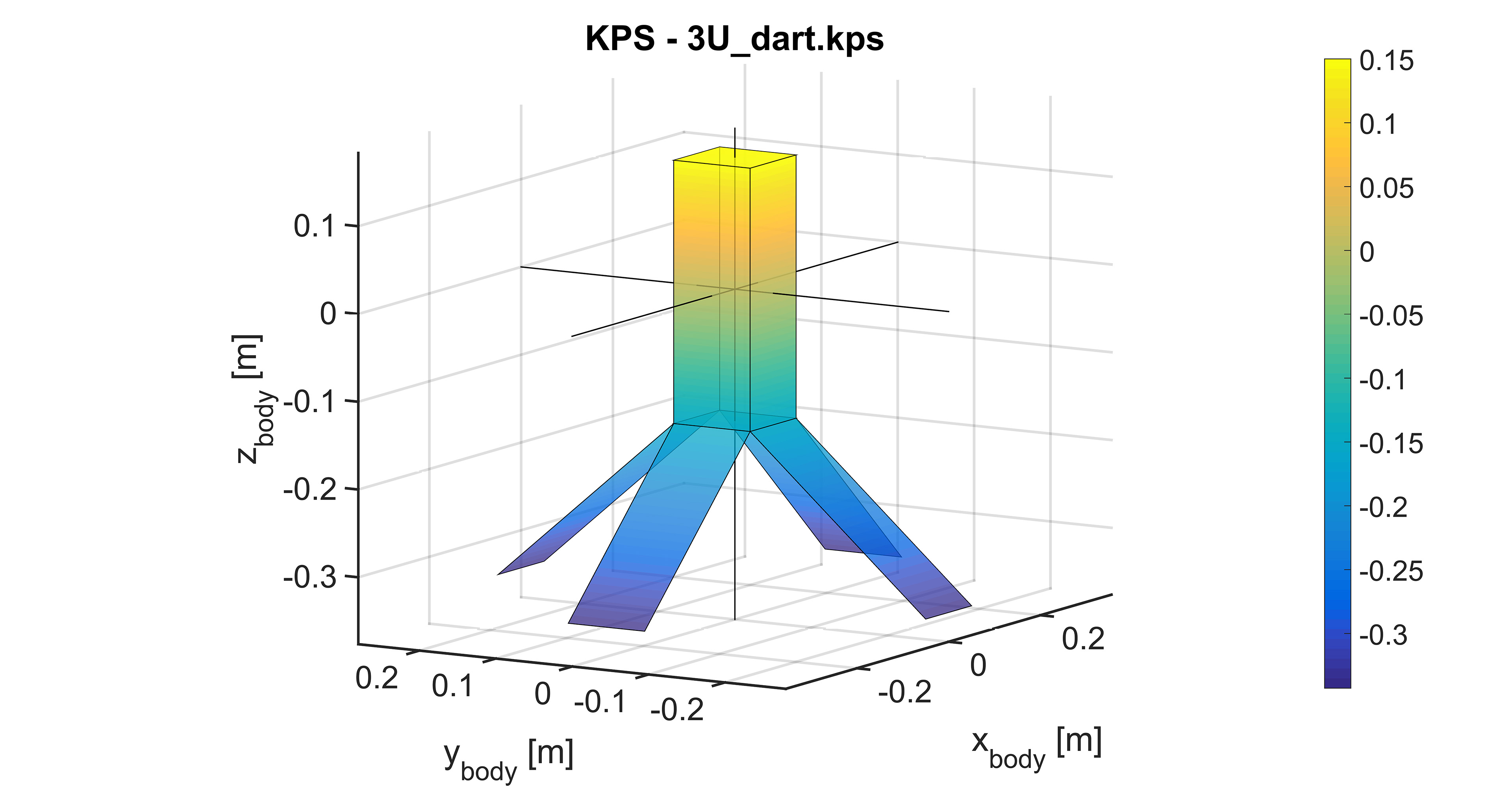
After producing a polygon file, the user should verify that the satellite has been described correctly. For this reason I provide the KPS_PlotPoly utility, which plots a KPS polygon file of the sort generated by KPS_GenPoly in 3-D for a user to inspect. It takes one argument – the name of the polygon file to load. It parses the file and produces an interactive 3-D plot for the user. This utility requires the matplotlib and numpy modules.
This utility allows users to convert Keplerian Elements to State Vectors. The utility takes the six Keplerian elements as arguments, as follows:
KPS_Kepler2State <a> <e> <w> <Omega> <i> <M>
The following table elaborates on each argument and its units:
| Argument | Name | Units |
|---|---|---|
| a | Semi-major Axis | Meters |
| e | Eccentricity | (Dimensionless) |
| i | Inclination | Degrees |
| Omega | RAAN or LAN | Degrees |
| w | Argument of Perigee | Degrees |
| M | Mean Anomaly | Degrees |
For example, the user might wish to experiment with propagating an existing satellite. The user can obtain the TLEs for that satellite from NORAD online and input the Kelperian elements into KPS_Kepler2State, obtain state vectors, and use the state vectors to start a KPS propagation run.
Example:
KPS_Kepler2State 6871000 0 45 0 0 0
The system responds:
Position Vector: 6871000, 0, 0 m
Velocity Vector: 0, 5385.7217960362, 5385.7217960362 m/s
This utility allows users to convert State Vectors to Keplerian Elements. One way to use the utility is to directly specify position and velocity vectors, in that order. The utility returns the six Keplerian elements (and some additional ones). The MATLAB version directly takes vectors:
KPS_State2Kepler([6871000, 0, 0], [0, 5385, 5385])
The Python version takes the same arguments, but split up into six scalars:
KPS_State2Kepler 6871000 0 0 0 5385 5385
In either case, the system responds:
True Anomaly: 0°
Mean Anomaly: 0°
Eccentric Anomaly: 0°
Semi-major Axis: 6871000.0015514 m
Eccentricity: 2.2579582648063e-10
Argument of Periapsis: 0°
Longitude of Ascending Node: 0°
Inclination: 45°
There is however, a second way to call the utility. The user can specify just a single argument – a time, in seconds. KPS_State2Kepler will search through the most recent KPS simulation run and find the first step time at or after that value. The utility will extract the position and velocity at that time and convert it to Keplerian elements. Note that this option requires the numpy module.
For example:
KPS_State2Kepler 500
The system responds:
Time: 500.02489376158 s
Position Vector: 5840925.18459, 2557032.12153, 2556656.26142 m
Velocity Vector: -4013.6839168, 4578.4141753, 4576.2060569 m/s
True Anomaly: 255.25022284075°
Mean Anomaly: -104.66942826045°
Eccentric Anomaly: -104.70960455682°
Semi-major Axis: 6868328.9059404 m
Eccentricity: 0.00072496937822618 m
Argument of Periapsis: 136.51435783804°
Longitude of Ascending Node: 359.99391990602°
Inclination: 44.988845461891°
The user runs KPS as follows:
KPS config.kps
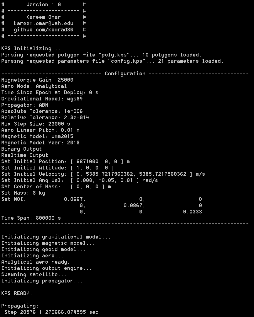
The system responds by echoing the parameters and other diagnostic information. If AERO_MODE is set to ANALYTICAL, the aerodynamics module reports analytical-mode initialization:
Initializing aero...
Analytical aero ready.
If AERO_MODE is set to GRID, the aerodynamics module reports grid initialization:
Initializing aero...
Grid aero ready.
If all initialization is successful, the system reports:
KPS READY.
Propagation begins:
Propagating:
 Step 37878 | 17042.926685 sec
The counter updates in real-time with the current step count and the number of seconds of orbit simulated. Propagation continues until the TIME_SPAN requested in the configuration file is achieved, or until satellite deorbit occurs, whichever comes first. Upon completion, the system displays:
Step 25054 | 10000.000000 sec
Propagation complete in 5.522 sec realtime.
Or, if deorbit occurred:
Step 9448 | 63.861708 sec
Satellite DEORBITED! Propagation complete in 3.423 sec realtime.
Or, if the user aborted propagation:
Step 3165 | 1044.177229 sec
Propagation terminated by user after 0.749 sec realtime.
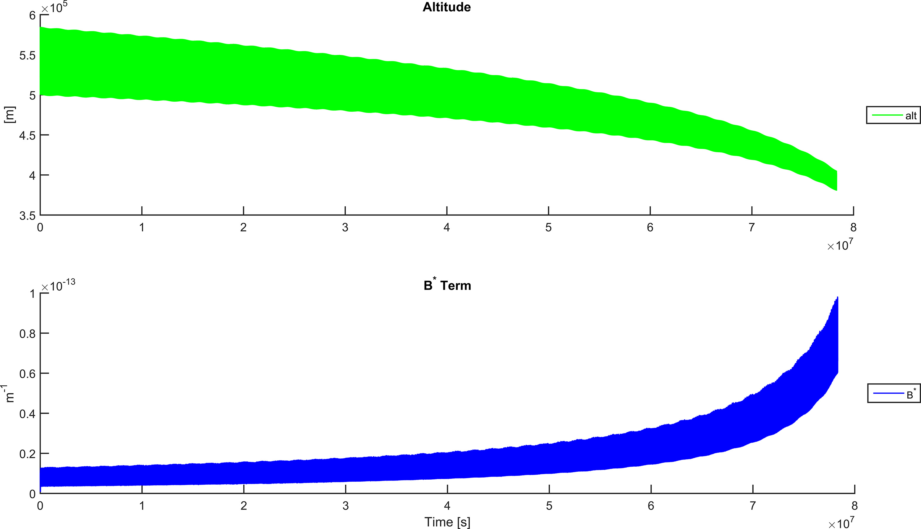
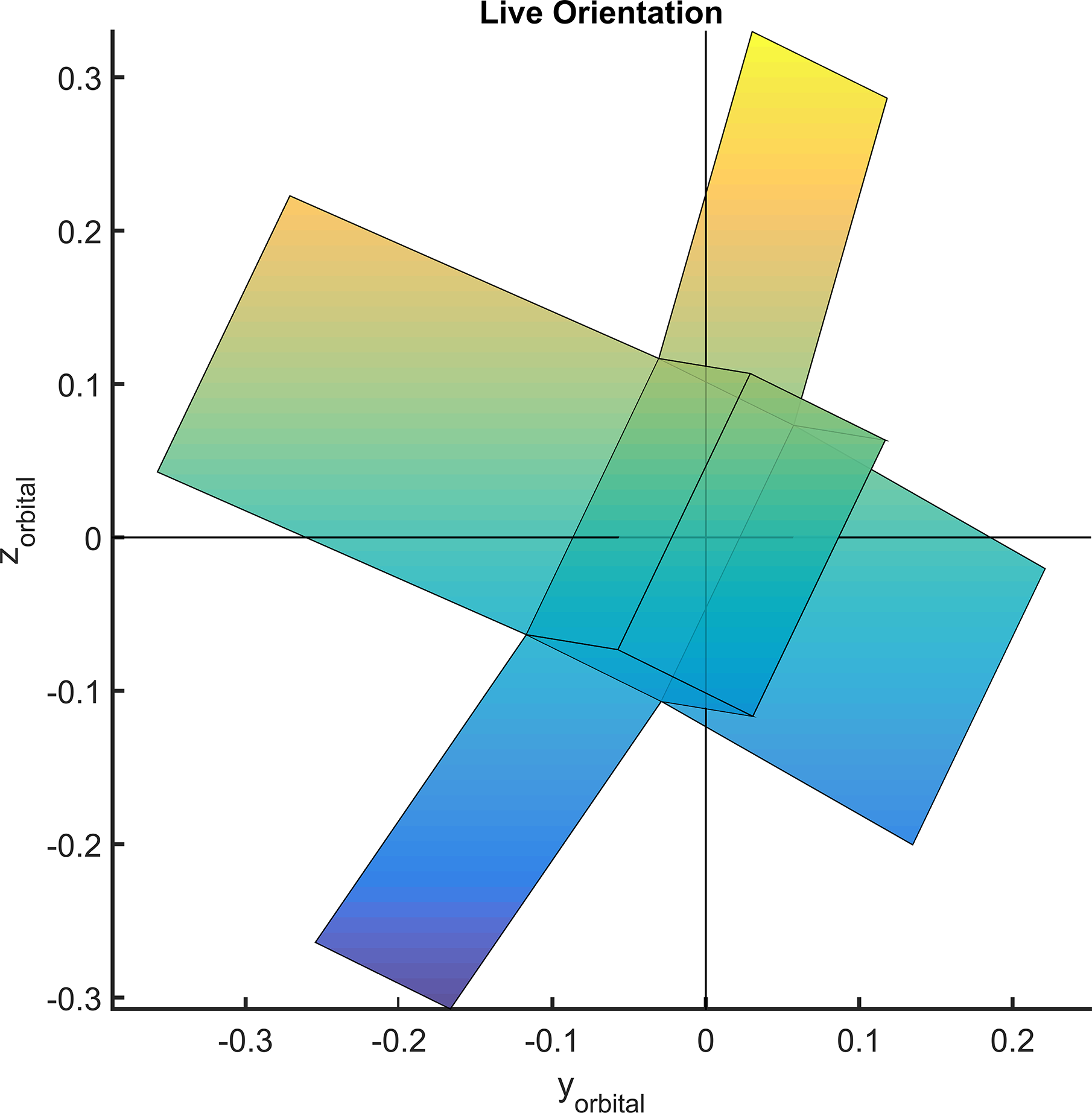
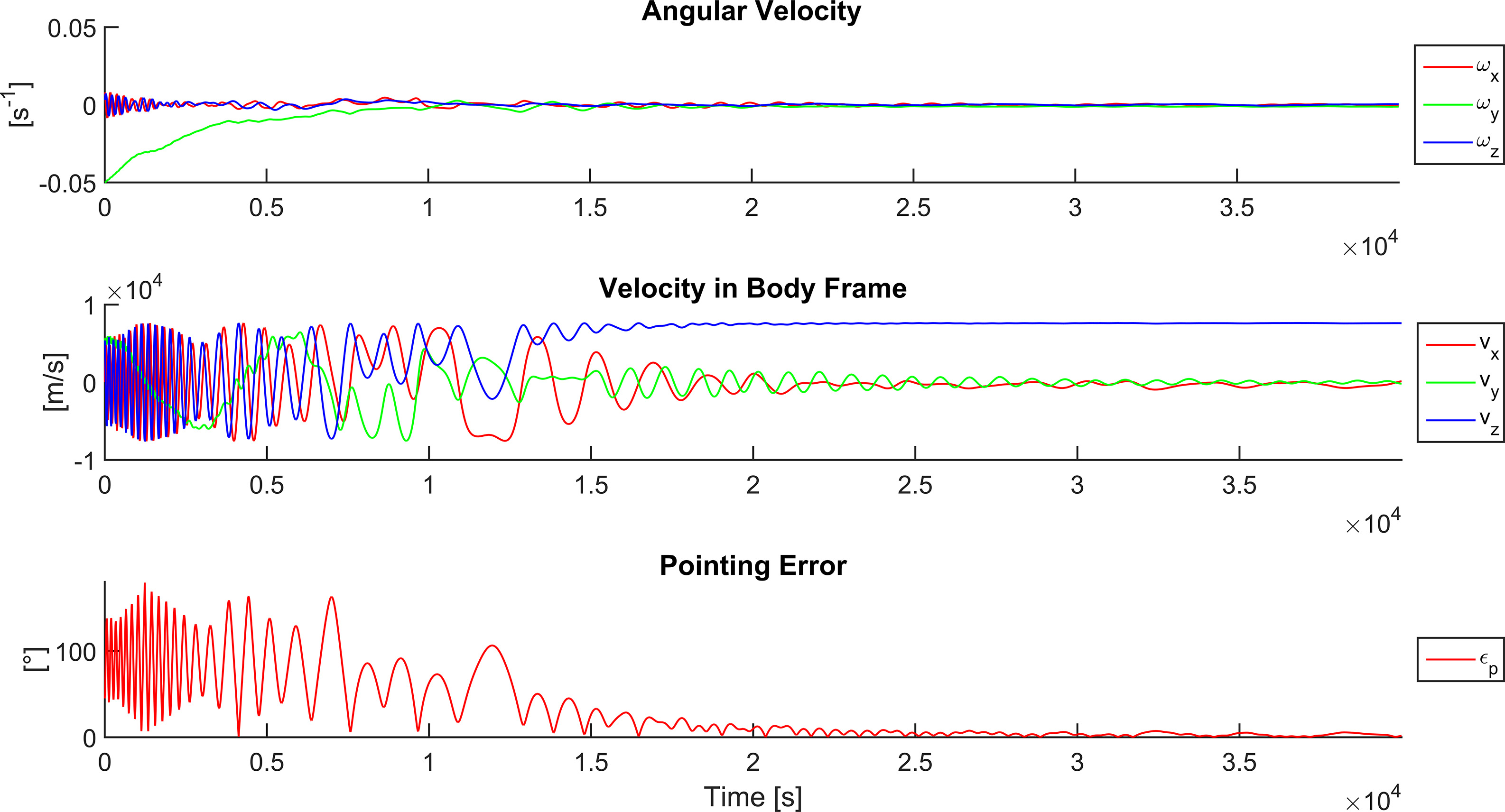
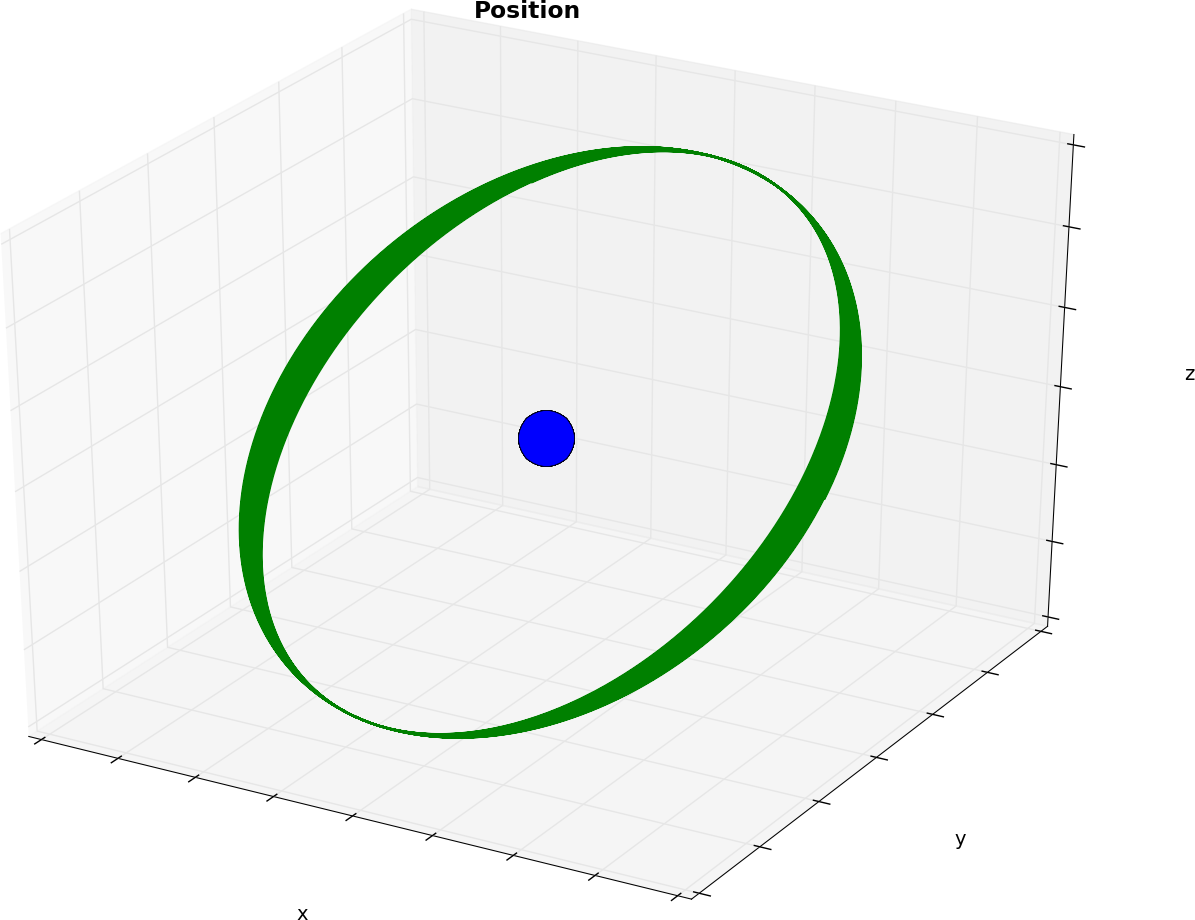
The fun part! While KPS is simulating, or afterward (the files are saved to disk), any combination of 18 satellite parameters can be plotted by KPS_Vis. The following table explains the available parameters:
| Parameter | Description |
|---|---|
| R | Position |
| ORIENTATION | Live 3-D View of Satellite Polygons |
| V | Velocity |
| Q | Attitude Quaternion |
| Q_ORB | Quaternion to Orbital Frame |
| ALT | Altitude |
| B_STAR | Starred Ballistic Coefficient |
| W | Angular Velocity |
| V_B | Velocity (in Body Frame) |
| E | Pointing Error |
| SEMI_MAJOR | Semi-major Axis |
| ECC | Eccentricity |
| INC | Inclination |
| RAAN | Right Ascension of Ascending Node |
| PERIAPSIS | Argument of Periapsis |
| MEAN_ANOM | Mean Anomaly |
| TRUE_ANOM | True Anomaly |
| ECC_ANOM | Eccentric Anomaly |
Simply choose Python (KPS_Vis.pyw) or MATLAB/Octave (KPS_Vis.m) and open the file for editing. Near the top you will see the list of available parameters. Don’t delete any lines or set any of them to ‘false’; just comment out the ones you don’t want to see, leaving only those you do. For example, the top of the MATLAB version shows:
plots = [
% R
ORIENTATION
% V
% Q
% Q_ORB
% ALT
% B_STAR
% W
% V_B
E
% SEMI_MAJOR
% ECC
% INC
% RAAN
% PERIAPSIS
% MEAN_ANOM
% TRUE_ANOM
% ECC_ANOM
];
More than about 3 plots or so at one time will be too small to be useful. Choose the ones you want, then save the file and run the simulation in the same directory as the KPS output files! No arguments to the script are required.
The simulation starts in REALTIME mode, constantly checking for and adding any new data from the KPS output files. If it sees no change for a while, indicating that simulation has finished, it switches to FINAL mode, cleans up the plots, adjusts the axes, and enables interactive mode for the user, who is then free to zoom, scale, rotate, save plots to image files, etc. The Python version requires the matplotlib and numpy modules. Some example screenshots are included with KPS.
