In his article published on KDnuggets in 2017 George McIntire describes an experiment building a "fake news" classifier using a document-vector model and Naive Bayes approach. He reports an 88% accuracy when classifying a "fake news" dataset which he assembled from various sources. This of course immediately made me wonder if deep neural networks (DNNs) can do better and if the performance increase due to these deep learners is statistically significant compared to the performance of the Naive Bayes classifier.
In the original experiment McIntire constructed a Naive Bayes classifier to classify the articles in his dataset as "Real" or "Fake" news. As published on GitHub the McIntire's "fake news" dataset has 6335 news articles of which 3171 articles are "real news" and 3164 articles are "fake news". The dataset is well balanced with respect to the two classes.
Note: The dataset as published contains a few more articles but the 'text' field for those articles is empty. These articles were removed for the analysis here.
I recreated McIntire's experiment using the following,
- A Multinomial Naive Bayes classifier with all the defaults in tact.
- A binary document-vector model using the scikit-learn
CountVectorizer.
and obtained the following results,
- A 90% accuracy estimated with an 80-20 hold-out set.
- The 95% confidence interval for the accuracy is [88%, 91%].
This very much validates the results that McIntire reports. Details of my recreation of McIntire's experiment can be found in the Python Jupyter notebook in my GitHub repository for this project. If you are not familiar with some of these concepts talked about here check out this tutorial on document classification.
In the document vector model of a collection of documents each word that appears in the collection is defined as a dimension in the corresponding vector model. Consider the following figure,
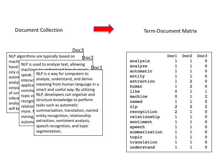
Here each column represents the feature vector of one of the documents in the collection and the rows are the features or dimensions of the vectors. Notice that there is one feature for each word that appears in the collection of documents. The column vectors can be fed to a classification algorithm for training. Here, the fields in the matrix are the counts of how many times a word appears in a document. However, there are many ways to encode the occurences of words in the collection within this matrix. In the binary CountVectorizer used in the experiment above the fields are just 0 and 1 indicating whether a particular word appears in a document or not. Perhaps the most famous encoding is TF-IDF, short for term frequency–inverse document frequency.
The vector representation of documents has two important consequences for document classification problems: The order and contexts of words are lost and semantic similarities between words cannot be represented. To see the importance of semantic similarity consider one document that discusses dogs and another document that discusses puppies. From a vector model perspective the feature set for these two documents will not intersect in terms of the notion of dog because the vector model simply considers dogs and puppies to be two different features and the similarity of these documents will not be apparent to a machine learning algorithm. To see the importance of the word context consider these two sentences: “it was not good, it was actually quite bad” and “it was not bad, it was actually quite good”. The vector representation of these sentences is exactly the same but they obviously have very different meanings or classifications. The vector representation of documents is often called the bag of words representation referring to the fact that it loses all order and context information.
Deep neural networks take a very different approach to document classification. Firstly, words are represented as embedding vectors with the idea that two words that are semantically similar to each other have similar vectors. Consider the following figure,

This figure represents a 3D embedding space and we can see that concepts that are similar to each other are close together in this embedding space. Therefore the similarity of our two documents talking about dogs and puppies will be recognized by a deep neural network aiding in the accuracy of a document classifier based on a DNN.
Secondly, in deep neural networks documents are no longer compressed into a vector representation of just word occurences. Instead, deep neural networks process actual sequences of words (coded as a integers) as they appear in the documents thereby maintaining the order and contexts of words. Consider the following code snippet using the Keras tokenizer applied to our two sentences from above,
from keras.preprocessing.text import Tokenizer
tok = Tokenizer()
# train tokenizer
tok.fit_on_texts(["it was not good, it was actually quite bad"])
# print sequences
print(tok.texts_to_sequences(["it was not good, it was actually quite bad"])[0])
print(tok.texts_to_sequences(["it was not bad, it was actually quite good"])[0])
This will print out the following sequences,
[1, 2, 3, 4, 1, 2, 5, 6, 7]
[1, 2, 3, 7, 1, 2, 5, 6, 4]
with a word_index of,
{'it': 1, 'was': 2, 'not': 3, 'good': 4, 'actually': 5, 'quite': 6, 'bad': 7}
These sequences can be directly fed into a deep neural network for training and classification. Notice that word order and context are nicely preserved in this representation.
The deep neural network we are using for our experiment can be seen here as a Python implementation using the Keras deep learning library,
from keras import layers
from keras.models import Sequential

model = Sequential(
    [
        # part 1: word and sequence processing
        layers.Embedding(num_words,
                         EMBEDDING_DIM,
                         input_length=MAX_SEQUENCE_LENGTH,
                         trainable=True),
        layers.Conv1D(128, 5, activation='relu'),
        layers.GlobalMaxPooling1D(),

        # part 2: classification
        layers.Dense(128, activation='relu'),
        layers.Dense(1, activation='sigmoid')
    ])

model.compile(loss='binary_crossentropy',
              optimizer='rmsprop',
              metrics=['accuracy'])
Our DNN can be broken down into two distinct parts. The first part consists of three layers and is responsible for word and sequence processing:
- The Embedding layer - learn word embeddings.
- The Convolution layer - learn patterns throughout the text sequences.
- The Pooling layer - filter out the interesting sequence patterns.
The second part consists of two layers,
- A Dense layer with a ReLU activation function.
- A Dense layer (also the output layer) with a Sigmoid activation function.
This part of the DNN can be viewed as a traditional feed-foward, back-propagation neural network with one hidden layer operating on a feature vector of length 128 computed by the first part of the DNN. In order to see this perhaps a bit clearer, here is the summary of the DNN as compiled by Keras,
_________________________________________________________________
Layer (type)                 Output Shape              Param #
=================================================================
embedding_1 (Embedding)      (None, 5000, 300)         7500300
_________________________________________________________________
conv1d_1 (Conv1D)            (None, 4996, 128)         192128
_________________________________________________________________
global_max_pooling1d_1 (Glob (None, 128)               0
_________________________________________________________________
dense_1 (Dense)              (None, 128)               16512
_________________________________________________________________
dense_2 (Dense)              (None, 1)                 129
=================================================================
Total params: 7,709,069
Trainable params: 7,709,069
Non-trainable params: 0
_________________________________________________________________
The None in the Output Shape column simply denotes the current batch size default. That means the pooling layer computes a feature vector of size 128 which is passed into dense layers of the feedforward network as we mentioned above.
The overall structure of the DNN can be understood as a preprocessor defined in the first part that is being trained to map text sequences into feature vectors in such a way that the weights of the second part can be trained to obtain optimal classification results from the overall network.
I trained this network for 10 epochs with a batch size of 128 using a 80-20 training/hold-out set. A couple of notes on additional parameters: The vast majority of documents in this collection is of length 5000 or less. So for the maximum input sequence length for the DNN I chose 5000 words. There are roughly 100,000 unique words in this collection of documents. I arbitrarily limited the dictionary that the DNN can learn to 25% of that: 25,000 words. Finally, for the embedding dimension I chose 300 simply because that is the default embedding dimension for both word2vec and GloVe.
The results were quite impressive,
A 97% accuracy with a 95% confidence interval of [96%, 98%].
The performance increase is statistically significant compared to the performance of the Naive Bayes classifier and perhaps a bit surprising given the relative simplicity of the DNN. One conclusion that one might draw is that semantic similarity between words and word order or context are crucial for document classification.