NordicSMC Winter School 2009
Overview:
- First steps
- SigMinr Part I: signal analysis
- Useful general tricks
- AudMinr: audio analysis
- MusMinr: music analysis
- SigMinr Part II
- PhyMinr: motion capture and physics
- VidMinr: video analysis
Download the latest repository version of the MiningSuite, available here.
If you run Matlab via the ProgramKiosk, you need to download MiningSuite from the link above using Internet Explorer directly in the ProgramKiosk.
Extract the miningsuite-master.zip file. You get a miningsuite-master folder which contains itself another miningsuite-master subfolder. To avoid confusion, rename that subfolder simply miningsuite. You can move that folder anywhere you like in your computer (or in your drive on the ProgramKiosk).
Add that miningsuite folder to your Matlab path.
Now if you write help miningsuite in the Command Window in Matlab and press enter, you should see the list of operators available in the MiningSuite.
The MiningSuite is decomposed into a certain number of packages (SigMinr, AudMinr, etc.) and in order to call an operator of a given package, you need to specify the package it belongs to, by adding the proper prefix.
For instance sig.signal is an operator from the SigMinr package, as indicated by the prefix sig.
Each operator is related to a particular data type: for instance, sig.signal is related to the loading, transformation and display of signals. Let's first load a WAV file of name test.wav:
sig.signal('test.wav')
Operations and options to be applied are indicated by particular keywords, expressed as arguments of the functions. For instance, we can just extract a part of the file, for instance from 1 to 2 seconds:
sig.signal('test.wav','Extract',1,2)
Let's try another operator sig.spectrum, which will be explained in the next section:
sig.spectrum('test.wav')
We can store the result of one operation into a variable, for instance:
a = sig.signal('test.wav','Extract',1,2)
In this way, we can perform further operations on that result. For instance, playing the audio:
sig.play(a)
or computing sig.spectrum on that result:
sig.spectrum(a)
For more details about the basic principles of the MiningSuite, check this page.
You can load various type of audio files, for instance MP3:
sig.signal('beethoven.mp3')
You can also load other types of signals, for instance sensor data, here collected using a FLOW breathing sensor in the context of MusicLab Vol. 2. You can find both the audio recording (P2.wav) and the breath data (P2.csv) in this zip file.
p2 = sig.signal('P2.csv')
Only numerical fields are taken into consideration.
Various options are available, as detailed in the sig.signal online documentation.
We can play the audio recording of the piece P2 while looking at the breath curve (with a cursor progressively showing us the successive temporal positions in each curve).
First we need to sync together the sensor data and the audio recording. Corresponding sensor data and audio recordings do not start at the same time, so we need to indicate the delay between the two signals.
For instance, for the second piece in vol. 2, there is a 23 s delay of the audio with respect to the breath data. We can sync them together using this command:
t = sig.sync(p2,'P2.wav',23)
In this way, we can now play the two files in sync:
t.play
To see all the frequencies contained in your signal, use sig.spectrum:
sig.spectrum('test.wav')
You can select a particular range of frequencies:
sig.spectrum('test.wav','Min',10,'Max',1000)
To learn more about the maths behind this transformation, and all the possible options, check the sig.spectrum online documentation.
The analysis of a whole temporal signal leads to a global description of the average value of the feature under study. In order to take into account the dynamic evolution of the feature, the analysis has to be carried out on a short-term window that moves chronologically along the temporal signal. Each position of the window is called a frame. For instance:
f = sig.frame('test.wav','FrameSize',1,'Hop',0.5)
Then we can perform any computation on each of the successive frame easily. For instance, the computation of the spectrum for each successive frame, can be written as:
sig.spectrum(f,'Max',1000)
What you see in the progressive evolution of the spectrum over time, frame by frame. This is called a spectrogram.
More simply, you can compute the same thing by writing just one command:
sig.spectrum('test.wav','Max',1000,'Frame')
Here the frame size was chosen by default. You can of course specify the frame size yourself:
sig.spectrum('test.wav','Max',1000,'Frame','FrameSize',1,'Hop',0.5)
For more information about sig.frame, click on the link.
Once we have computed the spectrogram
s = sig.spectrum('test.wav','Frame')
we can evaluate how fast the signal changes from one frame to the next one by computing the spectral flux:
sig.flux(s)
In the resulting curve, you see peaks that indicate particular moments where the spectrum has changed a lot from one frame to the next one. In other words, those peaks indicate that something new has appeared at that particular moment.
You can compute spectral flux directly using the simple command:
sig.flux('test.wav')
The flux can be computed from other representations that the spectrum. For more information about sig.flux, click on the link.
You can get an average of the amplitude of the signal by computing its Root Mean Square (or RMS):
sig.rms('test.wav')
But this gives a single numerical value, which is not very informative (although you can compared different signals in this way).
You can also see the temporal evolution of this averaged amplitude by computing RMS frame by frame:
sig.rms('test.wav','Frame')
We have now seen two ways to detect new events in the signal: sig.flux considers the changes in the spectrum while sig.rms considers the contrasts in the amplitude of the signal.
For more information about sig.rms, click on the link.
From a signal can be computed the envelope, which shows the global outer shape of the signal.
e = sig.envelope('test.wav')
It is particularly useful in order to show the long term evolution of the signal, and has application in particular to the detection of events. So it is very closely related to sig.rms that we just saw.
You can listen to the envelope itself. This is played by a simple noise that follows exactly the same envelope.
sig.play(e)
sig.envelope can be estimated using a large range of techniques, and with a lot of parameters that can be tuned. For more information, click on the link.
For any kind of representation (curve, spectrogram, etc.) you can easily find the peaks showing the local maxima by calling sig.peaks. For instance, on the envelope we just computed:
sig.peaks(e)
You can specify that you just want the highest peak:
sig.peaks(e,'Total',1)
set some threshold, for instance selecting all peaks higher than half the maximum value:
sig.peaks(e,'Threshold',.5)
You can see that by default sig.peaks selects some peaks in a kind of adaptive way. You can turn off this adaptive peak picking by toggling off the 'Contrast' option:
sig.peaks(e,'Contrast',0)
For more information about sig.peaks, click on the link.
We saw that we can find all the frequencies in a signal by computing sig.spectrum. But it is actually focused on finding sinusoids. More generally, if you want to find any kind of periodicities in a signal, for instance our envelope we just computed, we can compute an autocorrelation function by using sig.autocor:
sig.autocor(e)
Each peak in the autocorrelation function indicates periodicities. But these periodicities are expressed as lags, which corresponds to the duration of one period. If you want to see instead periodicities as frequencies (similar to sig.spectrum), use the 'Freq' option:
sig.autocor(e,'Freq')
And again you can specify the range of frequencies. For instance:
sig.autocor(e,'Freq','Max',10,'Hz')
We can also analyse the sensor data.
sig.autocor(p2)
We can also detect the presence of periodicities locally at particular temporal regions in the signals. To do so, we can decompose the signal into frames and compute the autocorrelation function for each successive frame:
sig.autocor(p2,'FrameSize',10,'FrameHop',.1)
For more information about sig.autocor, click on the link.
We can also check if the breath signal of a participant (or musician) is similar to the breath signal of another participant. We can compute the cross-correlation between each pairs of those signals.
sig.crosscor(s)
Peaks in the crosscorrelation curves indicate that two participants have same behaviour, with a delay between each other indicated by the lag (X axis). These periodicities are estimated globally throughout the whole signals.
We can also detect the presence of similar behaviour between pairs of participants locally at particular temporal regions in the signals. To do so, we can decompose the signal into frames and compute the crosscorrelation function for each successive frame:
sig.crosscor(s,'Frame','FrameSize',20,'FrameHop',.1)
Here we indicate frames of 20 seconds, that moves every 10% of the frame length (hence 2 seconds).
Something more technical, not necessarily useful for you, but of interest for experts in signal processing. Here is an example of more complex operation that can be performed: the decomposition of the signal into different channels corresponding to different frequency regions:
f = sig.filterbank('test.wav','CutOff',[-Inf,1000,5000])
You can play each channel separately:
sig.play(f)
You can then compute any operation on each channel separately, for instance:
e = sig.envelope(f)
And you can finally sum back all the channels together:
e = sig.sum(e)
For more information about sig.filterbank, click on the link.
You can perform any operation to a whole folder of files. For instance, if you would like to analyse all the audio and text files available in the mining suite distribution, first select the miningsuite folder as your Current Folder in Matlab. Then Instead of writing the name of a particular file, write the 'Folder' keyword instead. For instance:
sig.spectrum('Folder')
This paragraph requires some basic knowledge of Matlab. If you are not familiar with Matlab, you can skip this for the moment.
You have noticed that every time you perform a command, you obtain either a graphic on a new window, or the display of a single value directly in Matlab's Command Window. But you can of course get the actual numerical results in a Matlab structure (an array, for instance).
For instance, if you store the result of your analysis in a variable:
a = sig.spectrum('test.wav')
Then you can use the following syntax to output the actual results in Matlab.
a.getdata
When extracting peaks:
p = sig.peaks(e)
you can get the position of each peak:
get(p,'PeakPos')
and the value associated to each peak:
get(p,'PeakVal')
More information in the Advanced use page.
Let's suppose we compute a series of operations such as the following:
f = sig.filterbank('test.wav','CutOff',[-Inf,1000,5000]);
e = sig.envelope(f);
s = sig.sum(e);
p = sig.peaks(s);
Then it is possible to see again the series of operations, with detailed information about all the parameters, by using the .show command:
p.show
Again for Matlab experienced users, you can import in the MiningSuite any data you have already computed in Matlab. For instance let's say we generate an array using this Matlab command:
c = rand(100,1)
Then we can import this array as values of sig.signal. Here you need to know that sig.signal actually outputs a Matlab object of class sig.Signal. So to create your own object, use the sig.Signal method:
sig.Signal(c)
You can specify the sampling rate:
sig.Signal(c,'Srate',100)
I have not yet added a proper documentation of those classes in the MiningSuite. Please use the discussion list if you have any question meanwhile.
So far we have considered the analysis of any kind of signals. Let's now focus on the analysis of audio files.
The file test.wav we were using previously turns out to be a mono file. If we load now a stereo file:
sig.signal('ragtime.wav')
We actually can see the left and right channels separately. Any type of analysis can then be performed on each channel separately:
sig.envelope('ragtime.wav')
But if you prefer considering the audio file as a simple signal, you can mix altogether the left and right channels into a single mono signal by using the 'Mix' option:
sig.signal('ragtime.wav','Mix')
The 'Mix' option can be used for any command:
sig.envelope('ragtime.wav','Mix')
We can extract the fundamental frequency of each sound in the recording by calling aud.pitch:
aud.pitch('voice.wav','Frame')
The algorithms used in aud.pitch are currently being improved. We see in the example that there are some spurious high frequencies detected that should not be there. One possible way to remove those high frequencies could be to constrain the frequencies to remain below a given threshold:
aud.pitch('voice.wav','Frame','Max',300)
Or we can just extract the most dominant pitch in each frame:
aud.pitch('voice.wav','Frame','Total',1)
It is also theoretically possible to detect multiple pitches, for instance in a chord made of several notes played simultaneously:
aud.pitch('chord.wav','Frame')
But again, please notice that the algorithms need to be improved. For more information about aud.pitch, click on the link.
One particular timbral quality of sounds is brightness, which relates to the relative amount of energy on high frequencies. This can be estimated using aud.brightness:
aud.brightness('beethoven.wav','Frame')
We can specify the frequency threshold, or cut-off, used for the estimation:
aud.brightness('beethoven.wav','Frame','CutOff',3000)
But again, please notice that the algorithms need to be improved. For more information about aud.brightness, click on the link.
There are many ways to describe timbre. One common description of timbre used in computer research is based on so called Mel-Frequency Cepstral Coefficients also simply known as MFCCs. It is somewhat tricky to understand what they really mean, but nevertheless it is a good way to compare different sounds or different frames based on their MFCCs. For instance:
aud.mfcc('george.wav','Frame')
For more information about aud.mfcc, click on the link.
By looking at the envelope of the signal (using sig.envelope, cf. above), we can estimate when each new sound event starts, as they usually correspond to peaks in the curve. Such event detection curve can be performed using aud.events, which uses this type of method, but optimised. For instance:
aud.events('voice.wav')
aud.events('test.wav')
We can also try to detect the attack phase of each event:
aud.events('test.wav','Attacks')
as well as the decay phase:
aud.events('test.wav','Decays')
We can then characterise these attack and decay phases as they play a role in the timbral characterisation of sounds:
- Duration of the attack and decay phases:
aud.attacktime('test.wav')
aud.decaytime('test.wav')
- Slope of the phases:
aud.attackslope('test.wav')
aud.decayslope('test.wav')
- Difference of amplitude at the beginning and end of these phases:
aud.attackleap('test.wav')
aud.decayleap('test.wav')
More details here.
One way of detecting rhythmical repetitions in an audio recording is based on fluctuation.
aud.fluctuation('test.wav')
We can see the frequency of the different repetitions for different registers, from low frequency (bottom line) to high frequency (top line). We can get a simplified representation by summing all the registers together:
aud.fluctuation('test.wav','Summary')
For more information about aud.fluctuation , click on the link.
To learn about the full list of operators available in AudMinr, click here.
You can load a MIDI file and display a piano-roll representation:
mus.score('song.mid')
You can select particular notes, for instance the first 10 ones:
mus.score('song.mid','Notes',1:10)
or the first 5 seconds:
mus.score('song.mid','EndTime',5)
An audio recording can also be transcribed into a score, although the methods are very simplistic for the moment:
mus.score('test.wav')
You can turn a MIDI representation into a signal that can then be further analysed using SigMinr. For instance let's extract the pitch curve from a melody:
p = mus.pitch('song.mid')
We can then compute the histogram of that curve:
sig.histogram(p)
Similarly, we can compute the pitch-interval between successive notes:
p = mus.pitch('song.mid','Inter')
and compute the histogram of this new curve:
sig.histogram(p)
If we sample the pitch curve regularly:
p = mus.pitch('song.mid','Sampling',.1)
we can then compute the autocorrelation function to detect if there is a periodic repetition in the pitch curve:
sig.autocor(p)
We can try to detect the tempo of a piece of music:
mus.tempo('test.wav')
This operations is performed more or less using operators we already studied above. So here is a simplified explanation:
- First extract the event detection curve using a particular method called
'Filter':
o = aud.events('test.wav','Filter')
- Compute the temporal differentiation of this curve to emphasise the ascending and descending phases:
do = aud.events(o,'Diff')
- Compute an autocorrelation to detect periodicities in the curve. We use a
'Resonance'option to emphasise particular frequencies that are easier to perceive:
ac = mus.autocor(do,'Resonance')
- And finally detect the highest peak, corresponding to the tempo:
pa = sig.peaks(ac,'Total',1)
We can estimate the temporal evolution of tempo by adding, as usual, the 'Frame' keyword:
mus.tempo('test.wav','Frame')
We can perform exactly the same type of operations directly from a MIDI file:
mus.tempo('song.mid','Frame')
For more information about mus.tempo, click on the link.
Using the method just described, we can also have an estimation whether or not the pulsation is clearly present in the recording or more subtle. This is called pulse clarity, represented by a value that is higher when the rhythmic periodicity is clearer.
mus.pulseclarity('test.wav')
mus.pulseclarity('test.wav','Frame')
mus.pulseclarity('song.mid')
For more information about mus.pulseclarity, click on the link.
Let's turn now to tonal analysis. We can first get an estimation of the distribution of pitch classes used in the audio recording by computing a chromagram:
mus.chromagram('ragtime.wav')
As usual this can be computed frame by frame:
mus.chromagram('ragtime.wav','Frame')
And we can do the same with MIDI files:
mus.chromagram('song.mid')
For more information about mus.chromagram, click on the link.
From the chromagram, we can also have an estimation of the key, or tonality, of the audio recording. The key strength curve indicates the probability of each possible key, major or minor:
mus.keystrength('ragtime.wav')
mus.keystrength('ragtime.wav','Frame')
mus.keystrength('song.mid')
For more information about mus.keystrength, click on the link.
The highest score, as found by mir.peaks, gives the best key candidate:
ks = mus.keystrength('ragtime.wav');
sig.peaks(ks,'Total',1)
This can be obtained directly by calling mirkey:
mus.key('ragtime.wav')
mus.key('ragtime.wav','Frame')
mus.key('song.mid')
For more information about mus.key, click on the link.
From the key strength curve, it is also possible to assess whether the mode is major or minor. Majorness gives a numerical value which is above 0 if it is major, and below 0 if it is minor.
mus.majorness('ragtime.wav')
mus.majorness('ragtime.wav','Frame')
mus.majorness('song.mid')
For more information about mus.majorness , click on the link.
A more complex representation of tonality is based on a projection on a key-based Self-Organized Matrix (SOM). You can see in the projection that the most probable key is shown in red.
mus.keysom('ragtime.wav')
mus.keysom('ragtime.wav','Frame')
mus.keysom('song.mid')
For more information about mus.keysom , click on the link.
Find the diatonic pitch representation (for each note: its letter and accident) corresponding to the MIDI sequence:
mus.score('song.mid','Spell')
Very rudimentary algorithm integrated for the moment.
Local grouping based on temporal proximity, shown in blue rectangles:
mus.score('song.mid','Spell','Group')
Try with other MIDI files such as auclair.mid and mozart.mid.
Show broderies (in red rectangles) and passing notes (in grey):
mus.score('song.mid','Spell','Group','Broderie','Passing')
Try with other MIDI files such as auclair.mid and mozart.mid.
Find repeated motifs in the MIDI file auclair.mid:
mus.score('auclair.mid','Motif')
In the previous example, the motivic analysis is carried out only on pitch and pitch intervals. Add rhythm:
mus.score('auclair.mid','Motif','Onset')
Do the same with the MIDI file mozart.mid:
mus.score('mozart.mid','Motif')
So far, the pitch analysis is made only on the chromatic MIDI pitch information. To add diatonic information, we need to add the pitch spelling:
mus.score('mozart.mid','Motif','Spell')
The local grouping can be used to construct the syntagmatic network, and find ornamented motifs:
mus.score('mozart.mid','Motif','Spell','Group')
The version of the motivic analysis algorithms currently integrated in the MiningSuite are just experimental tests.
From a spectrogram:
s = sig.spectrum('test.wav','Frame')
we can compute a self-similarity matrix that shows the structure of the audio recording:
sig.simatrix(s)
We can compute the same representation from other input analyses, such as MFCC:
m = aud.mfcc('george.wav','Frame')
sig.simatrix(m)
The structural analysis depends highly on the choice of frame length and hop factor for the frame decomposition:
m = aud.mfcc('george.wav','Frame','FrameLength',1,'Hop',.5)
sig.simatrix(m)
For more information about sig.simatrix, click on the link.
Let's consider again our self-similarity matrix:
s = sig.spectrum('test.wav','Frame')
sm = sig.simatrix(s)
We can see in the matrix a succession of blocs along the diagonals, indicating successive homogenous sections. We can automatically detect the temporal positions of those change of sections by computing a novelty curve:
n = sig.novelty(sm)
sig.peaks(n)
For more information about sig.novelty, click on the link.
The initial audio recording can then be segmented based on those segmentation points we have detected as peaks of the novelty curve:
n = sig.novelty(sm)
p = sig.peaks(n)
sg = sig.segment('test.wav',p)
We can listen to each successive segment separately:
sig.play(sg)
If we perform any of the MiningSuite operations on this segmented signal, the operations will be performed on each successive segment separately:
s = aud.mfcc(sg)
For more information about sig.segment, click on the link.
From a given computation in the MiningSuite, for instance:
s = sig.spectrum('test.wav')
we can compute various statistics:
- the average:
sig.mean(s) - the standard deviation:
sig.std(s) - the histogram:
sig.histogram(s) - distribution moments:
sig.centroid(s),sig.spread(s),sig.skewness(s),sig.kurtosis(s) - other description of the flatness of the distribution:
sig.flatness(s),sig.entropy(s)
More information about all these operators in the complete documentation
The PatMinr package is mainly a partial integration of the MoCap Toolbox.
Load a mocap file (from Qualisys) and visualise the movement (a person walking):
p = phy.point('walk.tsv')
You can turn off the display of the index numbers:
phy.pref('DisplayIndex',0)
p
By default, the motion visualisation is real-time. Frames of the video are dropped in order to ensure the real-time quality. You can toggle off the frame drop. Since all frames are displayed, the video is slower.
phy.pref('DropFrame',0)
p
To revert to default options:
phy.pref('Default')
Some markers positions were not properly recorded. The missing points can be reconstructed:
p = phy.point('walk.tsv','Fill')
The mocap data can be turned into a signal using sig.signal. Let's select marker #3 and the third spatial dimension:
s = sig.signal(p,'Point',3,'Dim',3)
We can select a particular point of time (or temporal region):
p = phy.point('walk.tsv','Fill','Extract',160,160,'sp')
The points can be connected together to form a stick figure:
load('+phy/private/mocap.mat')
p = phy.point('walk.tsv','Fill','Connect',mapar)
We can represent a dancing stick figure in a "velocity space":
d2 = phy.point('dance.tsv','Connect',mapar)
d2v = phy.point('dance.tsv','Velocity')
d2v = phy.point('dance.tsv','Velocity','Connect',mapar)
as well as an "acceleration space":
d2a = phy.point('dance.tsv','Acceleration','Connect',mapar)
We can observe the three figures (position, velocity, acceleration) synced together:
s = phy.sync(d2,d2v,d2a)
Here also we can observe this visualisation without dropping frames:
phy.pref('DropFrame',0)
s
phy.pref('Default')
We can represent the velocity and acceleration in a phase plane:
sv = sig.signal(d2v,'Point',[1;19;25],'Dim',3)
sa = sig.signal(d2a,'Point',[1;19;25],'Dim',3)
s = sig.sync(sv,sa)
s.phaseplane
By computing the norm of the velocity (considered here as a simple time derivation of the positions) and summing the values altogether, we compute the total distance traveled by each marker:
d2v = phy.point('dance.tsv','Velocity','Connect',mapar,'PerSecond',0,'Filter',0);
sv = sig.signal(d2v,'Point',[1;19;25])
n = sig.norm(sv,'Along','dim')
sig.cumsum(n)
We can use sig.autocor from SigMinr to detect periodicities in the movement:
d2m1 = sig.signal(d2,'Point',1)
sig.autocor(d2m1,'Max',2)
d2m1 = sig.signal(d2,'Point',1,'Dim',3)
sig.autocor(d2m1,'Max',2)
sig.autocor(d2m1,'Max',2,'Enhanced')
sig.autocor(d2m1,'Max',2,'Frame','FrameSize',2,'FrameHop',.25,'Enhanced')
We can use mus.tempo from MusMinr to perform tempo estimation on the movement:
[t ac] = mus.tempo(d2m1)
[t ac] = mus.tempo(d2m1,'Frame')
Any time of statistics can be performed on the temporal signals of each marker:
d = phy.point('dance.tsv');
sd = sig.signal(d,'Point',[1;19;25])
sig.std(sd)
sig.std(sd,'Frame','FrameSize',2,'FrameHop',.25)
Here is for instance a comparison of the vertical skewness of particular markers for dancing and walking figures:
sd = sig.signal(d,'Point',[1;9;19;21;25],'Dim',3)
w = phy.point('walk.tsv');
sw = sig.signal(w,'Point',[1;9;19;21;25],'Dim',3)
sig.skewness(sd,'Distribution')
sig.skewness(sw,'Distribution')
phy.segment transforms a trajectory of points into a temporal motion of interconnected segments.
segmindex = [0 0 8 7 6 0 8 7 6 13 12 10 11 3 2 1 11 3 2 1];
ss = phy.segment('walk.tsv',j2spar,segmindex,'Reduce',m2jpar,'Connect',japar,'Fill')
From that representation, we can compute for instance potential energy of each segment, and sum them together:
pe = phy.potenergy(ss)
sig.sum(pe,'Type','segment')
We are starting to add video analysis.
We can watch a video file:
vid.video('video.mp4')
We can detect the changes in the video over time:
vid.video('video.mp4','Motion')
For more information about vid.video , click on the link.