REANA example - "world population"

About

This REANA reproducible analysis example demonstrates how to use parametrised Jupyter notebook to analyse the world population evolution.

Analysis structure

Making a research data analysis reproducible basically means to provide "runnable recipes" addressing (1) where is the input data, (2) what software was used to analyse the data, (3) which computing environments were used to run the software and (4) which computational workflow steps were taken to run the analysis. This will permit to instantiate the analysis on the computational cloud and run the analysis to obtain (5) output results.

1. Input data

We shall use the following input dataset:

• World_historical_and_predicted_populations_in_percentage.csv

It contains historical and predicted world population numbers in CSV format and was compiled from Wikipedia.

2. Analysis code

We have developed a simple Jupyter notebook for illustration:

• worldpopulation.ipynb

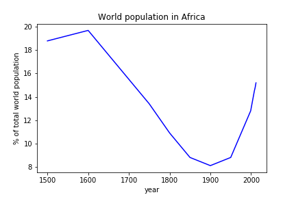
It studies the input dataset and prints a figure about how the world population evolved in the given region as a function of time.

The analysis code can be seen by browsing the above notebook.

3. Compute environment

In order to be able to rerun the analysis even several years in the future, we need to "encapsulate the current compute environment", for example to freeze the Jupyter notebook version and the notebook kernel that our analysis was using. We shall achieve this by preparing a Docker container image for our analysis steps.

Let us assume that we are using CentOS7 operating system and Jupyter Notebook 1.0 with IPython 5.0 kernel to run the above analysis on our laptop. We can use an already-prepared Docker image called reana-env-jupyter. Please have a look at that repository if you would like to create yours. Here it is enough to use this environment "as is" and simply mount our notebook code for execution.

4. Analysis workflow

This analysis is very simple because it consists basically of running only the notebook which will produce the final plot.

In order to ease the rerunning of the analysis with different parameters, we are using papermill to parametrise the notebook inputs.

The input parameters are located in a tagged cell and define:

• input_file - the location of the input CSV data file (see above)
• region - the region of teh world to analyse (e.g. Africa)
• year_min - starting year
• year_max - ending year
• output_file - the location where the final plot should be produced.

The workflow can be represented as follows:

           START
            |
            |
            V
+---------------------------+
| run parametrised notebook |  <-- input_file
|                           |  <-- region, year_min, year_max
|    $ papermill ...        |
+---------------------------+
            |
            | plot.png
            V
           STOP

For example:

$ papermill ./code/worldpopulation.ipynb /dev/null \
     -p input_file ./data/World_historical_and_predicted_populations_in_percentage.csv \
     -p output_file ./results/plot.png \
     -p region Europe \
     -p year_min 1600 \
     -p year_max 2010
$ ls -l results/plot.png

Note that we can also use CWL, Yadage or Snakemake : workflow specifications:

• workflow definition using CWL
• workflow definition using Yadage
• workflow definition using Snakemake

5. Output results

The example produces a plot representing the population of the given world region relative to the total world population as a function of time:

Running the example on REANA cloud

There are two ways to execute this analysis example on REANA.

If you would like to simply launch this analysis example on the REANA instance at CERN and inspect its results using the web interface, please click on one of the following badges, depending on which workflow system (CWL, Serial, Snakemake, Yadage) you would like to use:

If you would like a step-by-step guide on how to use the REANA command-line client to launch this analysis example, please read on.

We start by creating a reana.yaml file describing the above analysis structure with its inputs, code, runtime environment, computational workflow steps and expected outputs:

version: 0.3.0
inputs:
  files:
    - code/worldpopulation.ipynb
    - data/World_historical_and_predicted_populations_in_percentage.csv
  parameters:
    notebook: code/worldpopulation.ipynb
    input_file: data/World_historical_and_predicted_populations_in_percentage.csv
    output_file: results/plot.png
    region: Africa
    year_min: 1500
    year_max: 2012
workflow:
  type: serial
  specification:
    steps:
      - environment: 'docker.io/reanahub/reana-env-jupyter:2.0.0'
        commands:
          - mkdir -p results && papermill ${notebook} /dev/null -p input_file ${input_file} -p output_file ${output_file} -p region ${region} -p year_min ${year_min} -p year_max ${year_max}
outputs:
  files:
    - results/plot.png

In this example we are using a simple Serial workflow engine to represent our sequential computational workflow steps. Note that we can also use the CWL workflow specification (see reana-cwl.yaml), the Yadage workflow specification (see reana-yadage.yaml) or the Snakemake workflow specification (see reana-snakemake.yaml)).

We can now install the REANA command-line client, run the analysis and download the resulting plots:

$ # create new virtual environment
$ virtualenv ~/.virtualenvs/reana
$ source ~/.virtualenvs/reana/bin/activate
$ # install REANA client
$ pip install reana-client
$ # connect to some REANA cloud instance
$ export REANA_SERVER_URL=https://reana.cern.ch/
$ export REANA_ACCESS_TOKEN=XXXXXXX
$ # create new workflow
$ reana-client create -n myanalysis
$ export REANA_WORKON=myanalysis
$ # upload input code, data and workflow to the workspace
$ reana-client upload
$ # start computational workflow
$ reana-client start
$ # ... should be finished in about a minute
$ reana-client status
$ # list workspace files
$ reana-client ls
$ # download output results
$ reana-client download

Please see the REANA-Client documentation for more detailed explanation of typical reana-client usage scenarios.