Quickstart
In this tutorial, we assume that you already have installed Breeze.
Breeze is modeled on Scala, and so if you're familiar with it, you'll be familiar with Breeze. First, import the linear algebra package:
scala> import breeze.linalg._Let's create a vector:
scala> val x = DenseVector.zeros[Double](5)
x: breeze.linalg.DenseVector[Double] = DenseVector(0.0, 0.0, 0.0, 0.0, 0.0)
Here we make a column vector of zeros of type Double. And there are other ways we could create the vector - such as with a literal DenseVector(1,2,3) or with a call to fill or tabulate. The vector is "dense" because it is backed by an Array[Double], but could as well have created a SparseVector.zeros[Double](5), which would not allocate memory for zeros.
Unlike Scala, all Vectors are column vectors. Row vectors are represented as Transpose[Vector[T]].
The vector object supports accessing and updating data elements by their index in 0 to x.length-1. Like Numpy, negative indices are supported, with the semantics that for an index i < 0 we operate on the i-th element from the end (x(i) == x(x.length + i)).
scala> x(0)
Double = 0.0

scala> x(1) = 2

scala> x
breeze.linalg.DenseVector[Double] = DenseVector(0.0, 2.0, 0.0, 0.0, 0.0)
Breeze also supports slicing. Note that slices using a Range are much, much faster than those with an arbitrary sequence.
scala> x(3 to 4) := .5
breeze.linalg.DenseVector[Double] = DenseVector(0.5, 0.5)

scala> x
breeze.linalg.DenseVector[Double] = DenseVector(0.0, 2.0, 0.0, 0.5, 0.5)
The slice operator constructs a read-through and write-through view of the given elements in the underlying vector. You set its values using the vectorized-set operator :=. You could as well have set it to a compatibly sized Vector.
scala> x(0 to 1) := DenseVector(.1,.2)

scala> x
breeze.linalg.DenseVector[Double] = DenseVector(0.1, 0.2, 0.0, 0.5, 0.5)
Similarly, a DenseMatrix can be created with a constructor method call, and its elements can be accessed and updated.
scala> val m = DenseMatrix.zeros[Int](5,5)
m: breeze.linalg.DenseMatrix[Int] =
0  0  0  0  0
0  0  0  0  0
0  0  0  0  0
0  0  0  0  0
0  0  0  0  0
The columns of m can be accessed as DenseVectors, and the rows as DenseMatrices.
scala> (m.rows, m.cols)
(Int, Int) = (5,5)

scala> m(::,1)
breeze.linalg.DenseVector[Int] = DenseVector(0, 0, 0, 0, 0)

scala>  m(4,::) := DenseVector(1,2,3,4,5).t  // transpose to match row shape
breeze.linalg.DenseMatrix[Int] = 1  2  3  4  5

scala> m
breeze.linalg.DenseMatrix[Int] =
0  0  0  0  0
0  0  0  0  0
0  0  0  0  0
0  0  0  0  0
1  2  3  4  5
Assignments with incompatible cardinality or a larger numeric type won't compile.
scala> m := x
<console>:13: error: could not find implicit value for parameter op: breeze.linalg.operators.BinaryUpdateOp[breeze.linalg.DenseMatrix[Int],breeze.linalg.DenseVector[Double],breeze.linalg.operators.OpSet]
              m := x
                ^
Assignments with incompatible size will throw an exception:
scala> m := DenseMatrix.zeros[Int](3,3)
java.lang.IllegalArgumentException: requirement failed: Matrices must have same number of row
Sub-matrices can be sliced and updated, and literal matrices can be specified using a simple tuple-based syntax. Unlike Scalala, only range slices are supported, and only the columns (or rows for a transposed matrix) can have a Range step size different from 1.
scala> m(0 to 1, 0 to 1) := DenseMatrix((3,1),(-1,-2))
breeze.linalg.DenseMatrix[Int] =
3   1
-1  -2

scala> m
breeze.linalg.DenseMatrix[Int] =
3   1   0  0  0
-1  -2  0  0  0
0   0   0  0  0
0   0   0  0  0
1 2 3 4 5 All Tensors support a set of operators, similar to those used in Matlab or Numpy. See Linear Algebra Cheat-Sheet for a list of most of the operators and various operations. Some of the basic ones are reproduced here, to give you an idea.
| Operation | Breeze | Matlab | Numpy |
|---|---|---|---|
| Elementwise addition | a + b |
a + b |
a + b |
| Elementwise multiplication | a *:* b |
a .* b |
a * b |
| Elementwise comparison | a <:< b |
a < b (gives matrix of 1/0 instead of true/false) |
a < b |
| Inplace addition | a += 1.0 |
a += 1 |
a += 1 |
| Inplace elementwise multiplication | a :*= 2.0 |
a *= 2 |
a *= 2 |
| Vector dot product |
a dot b,a.t * b†
|
dot(a,b) |
dot(a,b) |
| Elementwise sum | sum(a) |
sum(sum(a)) |
a.sum() |
| Elementwise max | a.max |
max(a) |
a.max() |
| Elementwise argmax | argmax(a) |
argmax(a) |
a.argmax() |
| Ceiling | ceil(a) |
ceil(a) |
ceil(a) |
| Floor | floor(a) |
floor(a) |
floor(a) |
Sometimes we want to apply an operation to every row or column of a matrix, as a unit. For instance, you might want to compute the mean of each row, or add a vector to every column. Adapting a matrix so that operations can be applied column-wise or row-wise is called broadcasting. Languages like R and numpy automatically and implicitly do broadcasting, meaning they won't stop you if you accidentally add a matrix and a vector. In Breeze, you have to signal your intent using the broadcasting operator *. The * is meant to evoke "foreach" visually. Here are some examples:
scala> import breeze.stats.mean

scala> val dm = DenseMatrix((1.0,2.0,3.0),
                            (4.0,5.0,6.0))

scala> val res = dm(::, *) + DenseVector(3.0, 4.0)
breeze.linalg.DenseMatrix[Double] =
4.0  5.0  6.0
8.0  9.0  10.0

scala> res(::, *) := DenseVector(3.0, 4.0)

scala> res
breeze.linalg.DenseMatrix[Double] =
3.0  3.0  3.0
4.0  4.0  4.0

scala> mean(dm(*, ::))
breeze.linalg.DenseVector[Double] = DenseVector(2.0, 5.0)Breeze also provides a fairly large number of probability distributions. These mostly come with access to probability density function for either discrete or continuous distributions. Many distributions also have methods for giving the mean and the variance.
scala> import breeze.stats.distributions._

// As of Breeze 2, import this if you want "matlab"-like behavior with different random numbers from execution to execution
scala> import Rand.VariableSeed._

// As of Breeze 2, import this if you want consistent behavior with the same random numbers from execution to execution (modulo threading or other sources of nondeterminacy)
scala> import Rand.FixedSeed._

scala> val poi = new Poisson(3.0);
poi: breeze.stats.distributions.Poisson = <function1>

scala> val s = poi.sample(5);
s: IndexedSeq[Int] = Vector(5, 4, 5, 7, 4)

scala> s map { poi.probabilityOf(_) }
IndexedSeq[Double] = Vector(0.10081881344492458, 0.16803135574154085, 0.10081881344492458, 0.02160403145248382, 0.16803135574154085)

scala> val doublePoi = for(x <- poi) yield x.toDouble // meanAndVariance requires doubles, but Poisson samples over Ints
doublePoi: breeze.stats.distributions.Rand[Double] = breeze.stats.distributions.Rand$$anon$11@1b52e04

scala> breeze.stats.meanAndVariance(doublePoi.samples.take(1000));
breeze.stats.MeanAndVariance = MeanAndVariance(2.9960000000000067,2.9669509509509533,1000)

scala> (poi.mean,poi.variance)
(Double, Double) = (3.0,3.0)
NOTE: Below, there is a possibility of confusion for the term rate in the family of exponential distributions. Breeze parameterizes the distribution with the mean, but refers to it as the rate.
scala> val expo = new Exponential(0.5);
expo: breeze.stats.distributions.Exponential = Exponential(0.5)

scala> expo.rate
Double = 0.5
A characteristic of exponential distributions is its half-life, but we can compute the probability a value falls between any two numbers.
scala> expo.probability(0, log(2) * expo.rate)
Double = 0.5

scala> expo.probability(0.0, 1.5)
Double = 0.950212931632136
This means that approximately 95% of the draws from an exponential distribution fall between 0 and thrice the mean. We could have easily computed this with the cumulative distribution as well
scala> 1 - exp(-3.0)
Double = 0.950212931632136scala> val samples = expo.sample(2).sorted;
samples: IndexedSeq[Double] = Vector(1.1891135726280517, 2.325607782657507)
scala> expo.probability(samples(0), samples(1));
Double = 0.08316481553047272
scala> breeze.stats.meanAndVamake two objects for providing the random seed.riance(expo.samples.take(10000));
breeze.stats.MeanAndVariance = MeanAndVariance(2.029351863973081,4.163267835527843,10000)
scala> (1 / expo.rate, 1 / (expo.rate * expo.rate))
(Double, Double) = (2.0,4.0)TODO: document breeze.optimize.minimize, recommend that instead.
Breeze's optimization package includes several convex optimization routines and a simple linear program solver. Convex optimization routines typically take a
DiffFunction[T], which is a Function1 extended to have a gradientAt method, which returns the gradient at a particular point. Most routines will require
a breeze.linalg-enabled type: something like a Vector or a Counter.
Here's a simple DiffFunction: a parabola along each vector's coordinate.
scala> import breeze.optimize._

scala>  val f = new DiffFunction[DenseVector[Double]] {
     |               def calculate(x: DenseVector[Double]) = {
     |                 (norm((x - 3d) :^ 2d,1d),(x * 2d) - 6d);
     |               }
     |             }
f: java.lang.Object with breeze.optimize.DiffFunction[breeze.linalg.DenseVector[Double]] = $anon$1@617746b2
Note that this function takes its minimum when all values are 3. (It's just a parabola along each coordinate.)
scala> f.valueAt(DenseVector(3,3,3))
Double = 0.0

scala> f.gradientAt(DenseVector(3,0,1))
breeze.linalg.DenseVector[Double] = DenseVector(0.0, -6.0, -4.0)

scala>  f.calculate(DenseVector(0,0))
(Double, breeze.linalg.DenseVector[Double]) = (18.0,DenseVector(-6.0, -6.0))
You can also use approximate derivatives, if your function is easy enough to compute:
scala> def g(x: DenseVector[Double]) = (x - 3.0):^ 2.0 sum

scala> g(DenseVector(0.,0.,0.))
Double = 27.0

scala> val diffg = new ApproximateGradientFunction(g)

scala> diffg.gradientAt(DenseVector(3,0,1))
breeze.linalg.DenseVector[Double] = DenseVector(1.000000082740371E-5, -5.999990000127297, -3.999990000025377)
Ok, now let's optimize f. The easiest routine to use is just LBFGS, which is a quasi-Newton method that works well for most problems.
scala> val lbfgs = new LBFGS[DenseVector[Double]](maxIter=100, m=3) // m is the memory. anywhere between 3 and 7 is fine. The larger m, the more memory is needed.

scala> val optimum = lbfgs.minimize(f,DenseVector(0,0,0))
optimum: breeze.linalg.DenseVector[Double] = DenseVector(2.9999999999999973, 2.9999999999999973, 2.9999999999999973)

scala> f(optimum)
Double = 2.129924444096732E-29
That's pretty close to 0! You can also use a configurable optimizer, using FirstOrderMinimizer.OptParams. It takes several parameters:
case class OptParams(batchSize:Int = 512,
                     regularization: Double = 1.0,
                     alpha: Double = 0.5,
                     maxIterations:Int = -1,
                     useL1: Boolean = false,
                     tolerance:Double = 1E-4,
                     useStochastic: Boolean= false) {
  // ...
}
batchSize applies to BatchDiffFunctions, which support using small minibatches of a dataset. regularization integrates L2 or L1 (depending on useL1) regularization with constant lambda. alpha controls the initial stepsize for algorithms that need it. maxIterations is the maximum number of gradient steps to be taken (or -1 for until convergence). tolerance controls the sensitivity of the
convergence check. Finally, useStochastic determines whether or not batch functions should be optimized using a stochastic gradient algorithm (using small batches), or using LBFGS (using the entire dataset).
OptParams can be controlled using breeze.config.Configuration, which we described earlier.
We provide a DSL for solving linear programs, using Apache's Simplex Solver as the backend. This package isn't industrial strength yet by any means, but it's good for simple problems. The DSL is pretty simple:
import breeze.optimize.linear._
val lp = new LinearProgram()
import lp._
val x0 = Real()
val x1 = Real()
val x2 = Real()

val lpp =  ( (x0 +  x1 * 2 + x2 * 3 )
    subjectTo ( x0 * -1 + x1 + x2 <= 20)
    subjectTo ( x0 - x1 * 3 + x2 <= 30)
    subjectTo ( x0 <= 40 )
)

val result = maximize( lpp)

assert( norm(result.result - DenseVector(40.0,17.5,42.5), 2) < 1E-4)
We also have specialized routines for bipartite matching (KuhnMunkres and CompetitiveLinking) and flow problems.
**This API is highly experimental. It may change greatly. **
Breeze continues most of the functionality of Scalala's plotting facilities, though the API is somewhat different (in particular, more object oriented.) These methods are documented in scaladoc for the traits in the breeze.plot package object. First, let's plot some lines and save the image to file. All the actual plotting work is done by the excellent JFreeChart library.
import breeze.linalg._
import breeze.plot._

val f = Figure()
val p = f.subplot(0)
val x = linspace(0.0,1.0)
p += plot(x, x ^:^ 2.0)
p += plot(x, x ^:^ 3.0, '.')
p.xlabel = "x axis"
p.ylabel = "y axis"
f.saveas("lines.png") // save current figure as a .png, eps and pdf also supported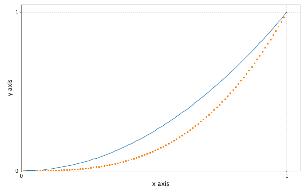
Then we'll add a new subplot and plot a histogram of 100,000 normally distributed random numbers into 100 buckets.
val p2 = f.subplot(2,1,1)
val g = breeze.stats.distributions.Gaussian(0,1)
p2 += hist(g.sample(100000),100)
p2.title = "A normal distribution"
f.saveas("subplots.png")
Breeze also supports the Matlab-like "image" command, here imaging a random matrix.
val f2 = Figure()
f2.subplot(0) += image(DenseMatrix.rand(200,200))
f2.saveas("image.png")
After reading this quickstart, you can go to other wiki pages, especially Linear Algebra Cheat-Sheet and Data Structures.