


Developed with the software and tools below.
In this computer vision tutorial using Python, we delve into image classification and segmentation. It is structured as five Jupyter notebooks, which you can follow along using an open dataset that contains images of trash.

This script provides two ways to download the TACO dataset for use in your project. The TACO dataset contains images and annotations used for training object detection models, specifically focused on trash classification.
Download Options
- Manual Download: This is the simpler option if you prefer to download the data yourself. The script provides a link to the TACO Kaggle repository where you can download the files. Once downloaded, you'll need to move them to a specific folder structure within your project directory (instructions provided in the code).
- Download using Kaggle API: This option automates the download process using Kaggle's API. Downloading the dataset through the Kaggle API can take some time due to its size (around 2.8 GB).
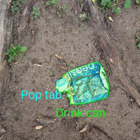
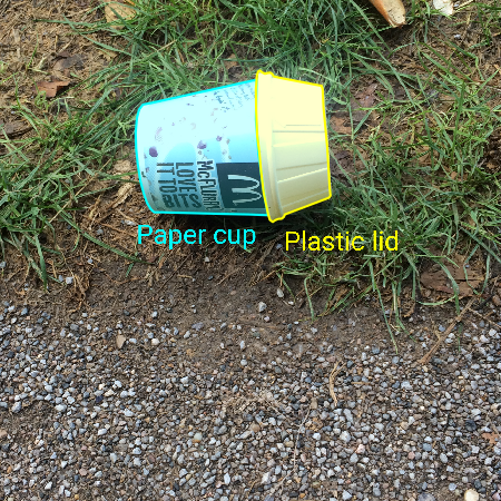
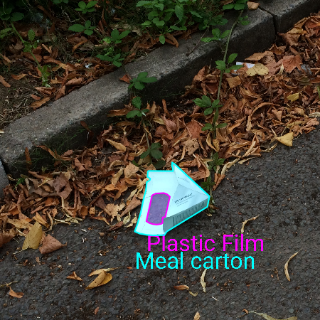
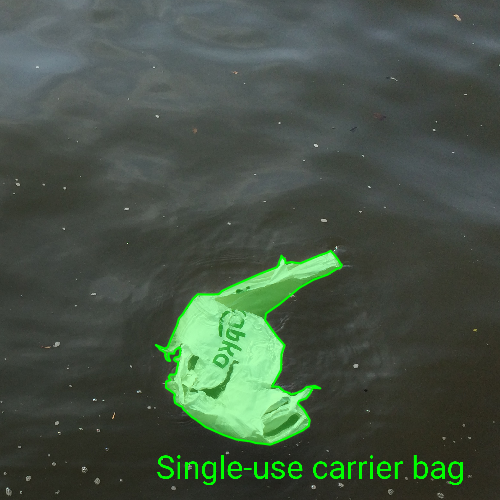
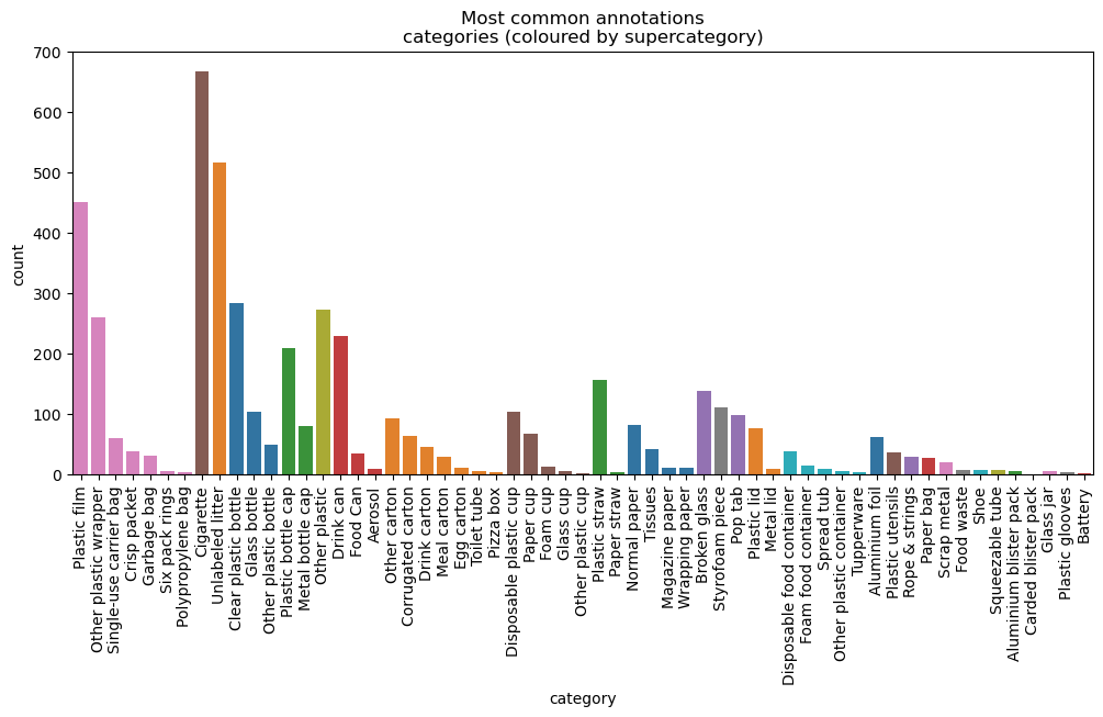
This notebook performs an exploratory data analysis (EDA) on the TACOdataset, which includes 1,500 crowd-sourced images of trash with COCO-Json annotations. This analysis helps understand the dataset's structure and prepares it for further machine learning tasks.
We start by loading the necessary libraries and defining paths for data. After loading the images and annotations, we analyzed the image metadata, checking for missing data and duplicates to ensure dataset integrity.
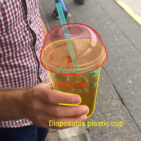
Next, we visualize random samples of annotations and analyzed their distribution by category and supercategory. This step highlighted the types of objects in the dataset and their frequencies.
We created class labels for five object types:
- Bottles
- Cartons
- Cups
- Cans
- Plastic Film
To prepare the images for machine learning, three main functions are defined. We load these from the helpers.py module.
show_annotation_imagedisplays the image containing the specified annotation.try_square_cropcrops the image around the annotation bounding box, with the crop size controlled by the widen_param.mask_and_square_cropcreates a mask image showing the contours of the annotation and crops this mask in the same way as the original image. This ensures that each processed image has a corresponding mask image with the same dimensions and object positioning.
The cropping function is demonstrated with various widen_param values, showing how the image is cropped more closely or broadly around the annotation.

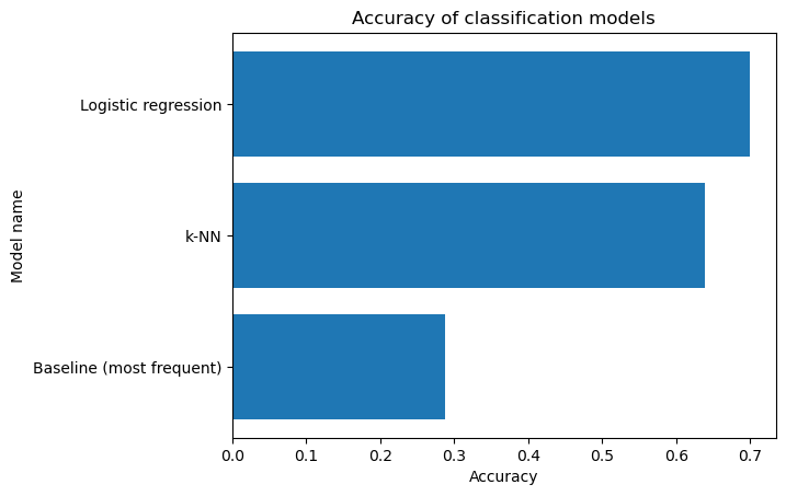
The dataset comprises 1,561 samples, with an unbalanced class distribution among the five classes. We use ResNet50V2, a pre-trained deep learning model designed for image classification tasks, to extract high-level features from the images. These features serve as the input for our machine learning models.
We use two different models for classification: K-nearest-neighbours and logistic regression. The baseline performance is established using a dummy classifier, which predicts the most frequent class. For the K-NN model, a grid search with cross-validation determines the optimal number of neighbors. For our logistic regression model, we use the 'one vs. rest' approach, incorporating an L2 penalty term to prevent overfitting and balancing class weights to mitigate class imbalance.
The accuracy of both models is summarised in the chart below.
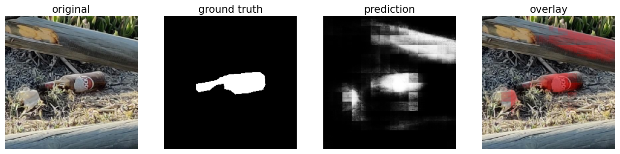
In this notebook, we we present an approach to image segmentation, focusing specifically on the identification of bottles within images. After loading necessary Python libraries, including keras_unet for image segmentation, we proceed to load the processed images and their corresponding masks. These masks delineate the regions of interest, namely the bottles, within the images.
For this purpose, we set up a Convolutional Neural Network (CNN) with a U-Net architecture for image segmentation. This architecture comprises contraction and expansive paths, designed to capture both local features and global context. To enhance model generalization and performance, we employ data augmentation techniques. Augmented images are generated to increase the diversity of the training dataset, thereby improving the model's ability to generalize to unseen data.
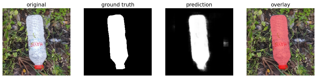
Following model training, we conduct performance assessment on the test set. We compare the trained model's predictions against ground truth masks using metrics such as Intersection over Union (IoU) to quantify segmentation accuracy. Here below, we display two predictions made by our model: one with a poor performance, where the contour of the bottle is difficult to make out against the object backgroun, and one where the contours of the bottle are almost perfectly predicted.
└── trash-images-analysis/
    ├── LICENSE
    ├── README.md
    ├── data
    │   ├── TACO
    │   │   └── data
    │   │	├──batch_1/
    │   │	├──batch_2/
    │   │	├──batch_3/
    │   │	├──batch_.../
    │   │	├──batch_15/
    │   │       └── annotations.json
    │   ├── features
    │   │   └── classification-labels.npz
    │   └── kaggle.json
    ├── environment.yml
    ├── helpers.py
    ├── notebooks
    │   ├── 00_download_data.ipynb
    │   ├── 01_exploratory_data_analysis.ipynb
    │   ├── 02_image_processing_for_ML_models.ipynb
    │   ├── 03_classifying_objects.ipynb
    │   └── 04_segmenting_images.ipynb
    └── saved_models
        └── widen_param_0.05
└── segm_model.h5helper functions and virtual environment setup
| File | Summary |
|---|---|
| helpers.py | helpers.py |
| environment.yml | environment.yml |
analysis notebooks
| File | Summary |
|---|---|
| 00_download_data.ipynb | notebooks/00_download_data.ipynb |
| 01_exploratory_data_analysis.ipynb | notebooks/01_exploratory_data_analysis.ipynb |
| 02_image_processing_for_ML_models.ipynb | notebooks/02_image_processing_for_ML_models |
| 03_classifying_objects.ipynb | notebooks/03_classifying_objects.ipynb |
| 04_segmenting_images.ipynb | notebooks/04_segmenting_images.ipynb |
Requirements
Ensure you have conda installed on your system before creating the environment. You can refer to the official conda documentation for installation instructions.
Ensure you have the following dependencies installed on your system:
- JupyterNotebook:
version v7.1.3
- Clone the trash-images-analysis repository:
git clone https://github.com/sg-peytrignet/trash-images-analysis- Change to the project directory:
cd trash-images-analysis- Install the dependencies with conda:
# We recommend installing the libmamba solver, which is faster
conda install -n base conda-libmamba-solver

# Create new environment called 'taco-env' with the required packages
conda env create -n taco-env -f environment.yml --solver mamba

# Activate the new environment
conda activate taco-envRun each notebook in the IDE of your choice, such as JupyterLab or Visual Studio.
To convert each notebook into an HTML document, run the command as show in the example below.
jupyter nbconvert 02_exploratory_data_analysis.ipynbContributions are welcome! Here are several ways you can contribute:
- Submit Pull Requests: Review open PRs, and submit your own PRs.
- Join the Discussions: Share your insights, provide feedback, or ask questions.
- Report Issues: Submit bugs found or log feature requests for Trash-images-analysis.
This project is protected under the MIT License.
- Thank you to the resources published by Dr. Sreenivas Bhattiprolu, which were useful to pre-process image data and annotations in the COCO-Json format.
- And thank you to my supervisors at the Ecole Polytechnique Federale de Lausanne for their guidance on carrying out this project.