The Select Link (SL) Module appends route information to microsimulated SWIM trips in order to create subarea external matrices. This is useful for creating external matrices for MPO models. A flow chart illustrating the SL module is shown below.

The select link module consists of two steps:
- Generate select link data
- Append select link data to trips
The first step takes select link locations (selectLinks.csv) as an input. This file is a mapping of SWIM network links to subarea network zones. For each link in the file, a select link analysis is run on the saved VISUM assignment paths. The assignment paths required for Select Link are generated during the SWIM Traffic Assignment (TA) module. If TA was not run, then the user needs to re-run the TA module in the desired year. The output from this step is a CSV file (selectLinkResults.csv) with the percent of OD demand using each select link. This file is essentially the tabular form of all the select link matrices generated by running a select link at each location. It is used to identify for each OD pair the share of demand using each select link. The file also contains the mapping of select link locations to subarea model station numbers for building subarea matrices later on.
The second step attaches the select link output (selectLinkResults.csv) to the trip lists output by the Person Transport (PT) and the Commercial Transport (CT) modules. Once the select link percent data has been appended to the trip lists, then various types of travel summaries can be prepared using the microsimulated trip list attributes. These summaries can include, for example, the commodities using a link(s) (or a screenline(s)), the household income distribution of all travelers using a link, subarea matrices by trip purpose, subarea matrices by truck class, etc.
The two steps are discussed in more detail below.
After paths are generated by the TA module, the SL module queries the path sets and stores select link volumes and flow matrices for each select link. Queries are run for each link in selectLinks.csv. An example selectLinks.csv file is shown in Inputs section.
The SL saves out ‘selectLinkResults.csv’ with the route share by assignment class, link fromnode, link tonode, link direction, origin, destination, and station number. The percent of demand using each select link is calculated by dividing the select link flow matrix value by the assigned demand for each OD, as shown below.

An example selectLinkResults.csv is shown in Outputs section.
The 'selectLinkResults.csv' identifies trips that are using the select link. However, it is also important to know where these trips would go if that link was not available. To help with such analysis, this step creates (sl.add.demand.matrices = true) separate OD matrices for select link demand and the remaining demand by vehicle class (auto or truck) and time period (peak, off-peak, pm, or ni). The remaining demand is calculated by subtracting the select link demand from the total demand. A user could disable the link and run assignment with the remaining demand segments (matrices) and see where the demand for that link is re-routed.
The demand matrices are added to a copy of the main version file (appends "_SL" to the file name). In all, 16 demand matrices are added to the new version file:
| Matrix Index | Matrix Name | Description |
|---|---|---|
| 21 | sl_d_offpeak | Select link truck demand in MD off-peak period |
| 22 | rem_d_offpeak | Remaining truck demand in MD off-peak period |
| 23 | sl_d_pm | Select link truck demand in PM period |
| 24 | rem_d_pm | Remaining truck demand in PM period |
| 25 | sl_a_peak | Select link auto demand in AM peak period |
| 26 | rem_a_peak | Remaining auto demand in AM peak period |
| 27 | sl_a_pm | Select link auto demand in PM period |
| 28 | rem_a_pm | Remaining auto demand in PM period |
| 29 | sl_a_offpeak | Select link auto demand in MD off-peak period |
| 30 | rem_a_offpeak | Remaining auto demand in MD off-peak period |
| 31 | sl_d_ni | Select link truck demand in NI period |
| 32 | rem_d_ni | Remaining truck demand in NI period |
| 33 | sl_d_peak | Select link truck demand in AM peak period |
| 34 | rem_d_peak | Remaining truck demand in AM peak period |
| 35 | sl_a_ni | Select link auto demand in NI period |
| 36 | rem_a_ni | Remaining auto demand in NI period |
To generate the 16 demand matrices, set 'sl.add.demand.matrices' to 'true' under select link properties in global properties.
This step can also assign select link and remaining demand to the network. To perform the assignment, the user needs to set 'sl.run.selectl.link.assignment' to 'true'. The assignment is performed for 4 classes of daily demand:
| Matrix Index | Matrix Name | Description |
|---|---|---|
| 37 | sl_a_daily | Daily select link auto demand |
| 38 | sl_d_daily | Daily select link truck demand |
| 39 | rem_a_daily | Daily remaining auto demand |
| 40 | rem_d_daily | Daily remaining truck demand |
It should be noted that when reviewing the properties file the user might also see a true/false titled 'sl.visum.mode'. This is an old legacy property that will not work in the "false" setting. So always leave set as true until the point at which the property can be removed which will allow this note to be removed.
The select link data is appended based on the type of select link analysis:
- Single link - if one link in selectLinks.csv
- Subarea - multiple links in selectLinks.csv enclosing a subarea
After calculating the OD share (percent) using each select link location (Generate Select Link Data), the results are then appended to the SWIM trip lists for SDT, LDT, CT, and ET. The auto (a) assignment class results are appended to the SDT and LDT tables, whereas the truck (d) assignment class results are appended to the CT and ET tables. Select link results are joined to the trip lists by assignment class, origin zone, and destination zone. Once joined, then the external station, percent/share, and link direction fields are also now attached to the trip lists. Trip records are duplicated if there is more than one path for the OD pair (i.e. more than one select link result of interest). When coding the trips, each select link location becomes a new origin or destination using the input station number as the zone number.
For this analysis, first select link percent data is appended to the trip lists (as described above in Single Link) and then subarea matrices by trip purpose, and time of day are created. Each microsimulated trip is converted to one of the following trips types in relation to the subarea (II, IE, EI, EE, IEI, and EXE).

If the select link Direction=IN then the link becomes a row (origin) in the subarea matrix. If the select link Direction=OUT then the link becomes a column (destination) in the subarea matrix. For example, a trip list record with appended select link percent for links with Direction=IN results in EI relations in the matrix. If a trip list record has 0 percent, then the OD pair is either II or EXE and is aggregated in the traditional manner.
It is fairly straightforward to convert the trip lists after the select links results data has been appended into subarea matrices. It gets a bit complicated when the path that a trip enters and exits the subarea more than once. These paths, called weaving paths, require special logic when converting them to matrix form. Before describing the weaving paths solution, the simpler cases are illustrated.
Below are examples of the II, IE, EI, and EE paths. The II path produces no select link results and therefore no matrix entries. The IE path produces a select link result for origin=A to destination=B via link=c and link=c is a direction=OUT link. The IE path produces two trips. The EI path produces two trips. The EE path produces three trips.


The weaving example (W) requires knowledge of the select link ordering in order to assign the trips to the matrix. As shown below, this is due to the fact that there are two direction=OUT links and it is not known which is the first out link so it can be “connected” to the origin zone.

The sequence of links for a given path between OD pairs are obtained from the path files generated by the TA module. Based on the link sequence, the link ordering is determined and the subarea matrix information can be coded. Currently only the shortest path between an OD given the calculated path set is used to determine the link ordering. This is almost always correct, but not guaranteed to be correct.
As illustrated in Outputs, the result is a zip file of SWIM trip lists with subarea matrix information appended to each record.
A summary of appended select link trips (sl.output.file.select.link.summary = sl_summary.csv) sl_summary.csv and an output with select link OD pairs to review (sl.output.file.select.link.review = sl_review.csv) sl_review.csv are also produced. These summary files contain trip counts of the appended trips and OD counts from selectLinkResults.csv respectively. The counts are summarized by time period (peak, offpeak, pm, ni), mode (auto, truck), station, and direction (IN, OUT). The review output contains OD pairs by time period and direction that do not add up to 100% for select link percent in the select link results file. These OD pairs should be reviewed to make sure that there are no issues in the select link results.
To run Select Link, the user needs to perform two steps:
- Setup Select Link
- Run Select Link
The Select Link module is setup through the tSteps.csv (under “/[scenario_name]/model/config”) file by turning on the following two properties in the desired year:
- SL - Generate Select Link Data
- SL - Append Select Link To Trips
To enable the two properties, edit the tsteps.csv file to contain a ‘1’ in the SL columns for each year where the user would like to run Select Link. For example, following setup runs SL in the year 20. The TA module needs to be run before running the SL in each year.

Also, in the properties file make sure that select link settings have demand segments and mode (auto and truck) segments set to four time periods, as below:
sl.visum.demand.segment.mapping = {'a_peak':1,'a_offpeak':2,'a_ni':3,'a_pm':4,'d_peak':5,'d_offpeak':6,'d_ni':7,'d_pm':8}
sl.auto.classes = a_peak,a_offpeak,a_pm,a_ni
sl.truck.classes = d_peak,d_offpeak,d_pm,d_ni
To run select link, first run the “/[scenario name]/build_run.bat” script. The script creates all of the necessary output folders and configuration files, as well as the batch files “/[scenario name]/run_model.bat” and “/[scenario name]/run_model_python.bat”.
Next, run the “run_model.bat” to start a model run. Running either of the two batch files will start the model run. Both batch files have identical functionality, only one is purely in batch form and the other runs through a Python layer. The reason both exist is that the former is simpler, but the latter may be needed if certain use cases arise in the future.
The SL module takes two input files:
- inputs\t0\selectLinks.csv
- inputs\t0\InternalZones.txt (optional)
The CSV file (selectLinks.csv) contains mapping of SWIM network links to subarea network zones. All SWIM links going in/out of the subarea needs to be mapped to SWIM zones, so that all trips would be captured. VISUM, ArcGIS, etc. can be used to map SWIM links to the external stations of the subarea.
The file must have at-least the following fields:
| FROMNODE | TONODE | DIRECTION | STATIONNUMBER |
|---|---|---|---|
| 15801 | 16091 | OUT | 1 |
| 16091 | 15801 | IN | 1 |
| 15980 | 16014 | IN | 4 |
| 16014 | 15980 | OUT | 4 |
FROMNODE and TONODE are SWIM links. The DIRECTION field means that the link is going into (IN) or out of (OUT) the selected area. The STATIONNUMBER is the external station number of the subarea (model).
There may be subarea external stations that do not map to a SWIM link. This may occur because SWIM statewide model has a coarser network and zone density than many urban models. Those links can be left out of the SWIM file. However, all SWIM links that enter/exit the subarea must be mapped to an external station or else trips will be lost.
The InternalZones.txt text file is an optional input that identifies the SWIM zones internal to the subarea. The format of the file is one zone number per row. It is used in the Append Select Link To Trips step to help define the subarea and to export II trips from SWIM for the subarea zones listed in the file. As a result, all SWIM zones that are internal to the subarea should be listed in the file if the II portion of the SWIM trip tables is desired.
Select link outputs are put in the scenario year-specific folder for each year: "[scenario name]\outputs[tstep]". The module outputs two files:
- selectLinkResults.csv
- select_link_outputs.zip
- sl_summary.csv
- sl_review.csv
The CSV file is an output of the first step of the SL module. The file contains the select link results in tabular form. A sample selectLinkResults.csv file is shown below.

Fields in selectLinkResults.csv are as in the table below.
| Field | Description |
|---|---|
| ASSIGNCLASS | Assignment class by time period (a_peak, a_offpeak, a_pm, a_ni, d_peak, d_offpeak, d_pm, d_ni) |
| FROMNODETONODE | SWIM link |
| DIRECTION | Link is going into (IN) or out of (OUT) the selected area |
| FROM ZONE | Origin Zone |
| TO ZONE | Destination Zone |
| PERCENT | Percent of demand using each select link |
| STATION NUMBER | External station number of the subarea (model) |
The ZIP file is an output of the second step of the SL module and contains the trips files with appended select link results. The ZIP file contains the following files:
- Trips_CTTruck_select_link.csv – subarea CT trips
- Trips_ETTruck_select_link.csv – subarea ET trips
- Trips_LDTPerson_select_link.csv – subarea LDT person trips
- Trips_SDTPerson_select_link.csv – subarea SDT trips
- SynPop_Taz_Summary.csv – SWIM zonal household and population data
- Employment.csv – SWIM zonal employment data by type
- Alpha2beta.csv – Alpha zone to beta zone correspondence
The output trip files contain the original file fields + five additional select link fields as shown in the table below. When a trip uses multiple external stations, the trip is duplicated in the trip lists when appending multiple select link percents.
| Field | Description |
|---|---|
| HOME_ZONE | Home location zone |
| EXTERNAL_ZONE_ORIGIN | External station if the trip is inbound to the subarea, else origin zone |
| EXTERNAL_ZONE_DESTINATION | External station if the trip is outbound to the subarea, else destination zone |
| SELECT_LINK_PERCENT | Percent of assigned traffic volume between the OD pair on the selected link (i.e. an external station) |
| FROM_TRIP_TYPE | if first trip on tour then (home or work) else previous trip purpose |
The CSV file summarizes counts of appended trips by station, direction (IN, OUT), and time period (peak, offpeak, pm, ni). The fields are as below:
| Field | Description |
|---|---|
| STATIONNUMBER | External station number of the subarea (model) |
| DIRECTION | Link is going into (IN) or out of (OUT) the selected area |
| PERIOD | Assignment class by time period (peak, offpeak, pm, ni) |
| AUTO_SL_OD | Count of OD pairs for auto trips |
| TRUCK_SL_OD | Count of OD pairs for truck trips |
| SDT_PERSON_TRIP | Count of SDT person trips |
| SDT_VEHICLE_TRIP | Count of SDT auto vehicle trips |
| LDT_PERSON_TRIP | Count of LDT person trips |
| LDT_VEHICLE_TRIP | Count of LDT auto vehicle trips |
| CT_TRIP | Count of CT trips |
| ET_TRIP | Count of ET trips |
The CSV file is produced only if there are suspect results from select link analysis. The file contains OD pairs by time period and direction that do not add up to 100% for select link percent in the select link results file. These OD pairs should be reviewed to make sure that there are no issues in the select link results. The fields are as below:
| Field | Description |
|---|---|
| ASSIGNCLASS | Assignment class by time period (a_peak, a_offpeak, a_pm, a_ni, d_peak, d_offpeak, d_pm, d_ni) |
| DIRECTION | Link is going into (IN) or out of (OUT) the selected area |
| origin | Origin zone |
| destination | Destination zone |
| SELECT_LINK_PERCENT | Percent of demand using each select link |
The figure and example selectLinkResults.csv table below illustrate how the SL module works. The figure shows seven select link locations that select a subarea for the Grants Pass, Medford, and Ashland area. The table includes entries for assignment class a_peak (PT demand) and d_peak (CT and ET (truck) demand). Origin zone 3175 is located NE of the subarea and destination zone 1735 is in Medford.
For the OD pair, the SL module reports that 100% of the auto demand entered through station 3. As shown in the Figure, for truck demand, SL reports that 91.3% of the demand entered through station 3 and the remaining (8.7%) through station 4. The shares are calculated by taking the total demand in the OD pair for each select link's matrix and dividing it by the total demand for the OD pair. There is one route for auto and two routes for truck because that's what VISUM calculated. Usually there is only one route and the total share of trips through a select link / external station is 100%.
| ASSIGNCLASS | FROMNODETONODE | DIRECTION | FROMZONE | TOZONE | PERCENT | STATIONNUMBER | SELECT_LINK_DEMAND | TOTAL_DEMAND |
|---|---|---|---|---|---|---|---|---|
| a_peak | 11555 11554 | IN | 3175 | 1735 | 1.000 | 3 | 1.000 | 1 |
| d_peak | 11555 11554 | IN | 3175 | 1735 | 0.913 | 3 | 0.913 | 1 |
| d_peak | 15066 15065 | IN | 3175 | 1735 | 0.087 | 4 | 0.087 | 1 |

The outputs of the SL module can be used to identify the pattern of trips entering and exiting the subarea. Desire line plots are a nice way to quickly visualize directionality and magnitude of trips using the sub-area. To demonstrate, six desire line plots of auto trips and truck trips are presented below. The plots also show populated places in the subarea. Darker gray color represents more population. The desire lines are labeled with the number of trips for the OD pair.
Auto Trips Entering (IN) at Station 1

Auto Trips Exiting (OUT) at Station 1

Auto Trips Entering (IN) at Station 7

Auto Trips Exiting (OUT) at Station 7
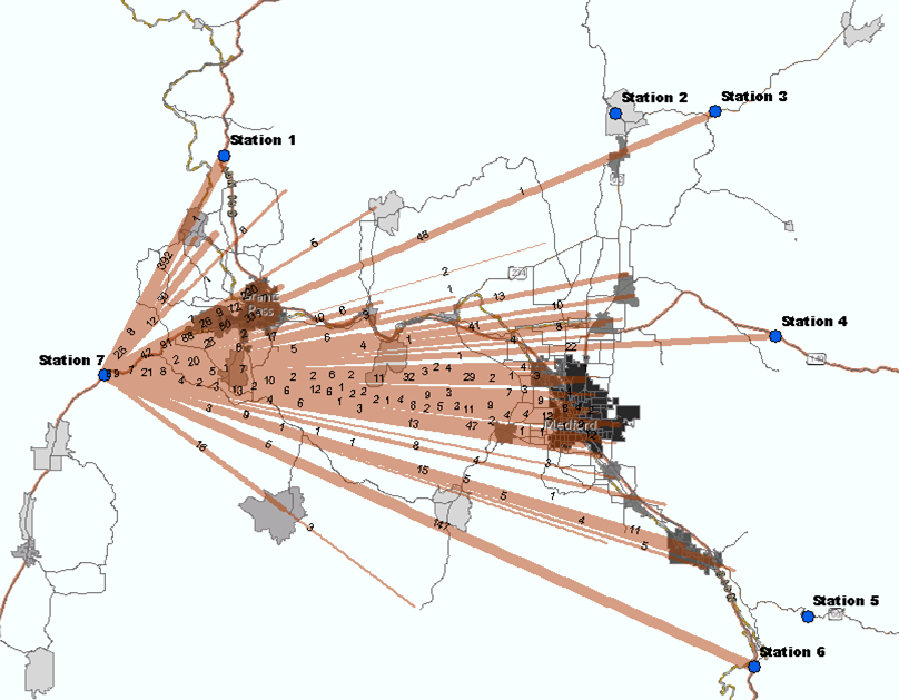
In general, the patterns of auto trips appear reasonable. The trips are travelling to/from populated places and the urban areas (Medford and Grants Pass) are getting a larger share of the trips. The plots show the importance of the interstate (I-5) in the subarea. The trips are predominantly using the interstate to travel between towns and external places.
Truck Trips Entering (IN) at Station 1

Truck Trips Leaving (OUT) at Station 1

As expected, truck trips at station 1 use the interstate to enter and exit the subarea. The interstate runs through the subarea and connects station 1 and station 6. A large portion of the truck trips are using the interstate to travel between the two stations, which shows how significant external-external truck trips are in the region.