Hnsw Real time Index Detailed Design
Hierarchical NSW Algorithm, is a new graph algorithm for approximate k nearest neighbor search. It is an improvement of the NSW (Navigable-Small-World-Graph) method, which consists of multiple layers of adjacent graphs, so it is called the hierarchical NSW method. It has the characteristics of high query accuracy and fast query speed, and also has a good effect on high-dimensional data. But whether it is the original author's open source HNSW algorithm hnswlib https://github.com/nmslib/hnswlib, or the classic similar search library faiss hnsw https://github.com/facebookresearch/faiss and other algorithms, none of them achieve real-time. The HNSW algorithm cannot be queried when constructing the index, so the query will be restricted. Therefore, it is necessary to implement the real-time HNSW algorithm. The following introduces the real-time HNSW algorithm implemented in vearch https://github.com/vearch/vearch, so that insertion and search can be performed at the same time, so that queries can also be performed when building the index.
NSW solves the problem of divergent search of neighbor graphs by designing a navigable graph, but its search complexity is still too high, reaching the level of multiple logarithms, and the overall performance is easily affected by the size of the graph. HNSW combined the skip-list idea on this basis and proposed a hierarchical structure. The structure of HNSW is shown in the figure below:
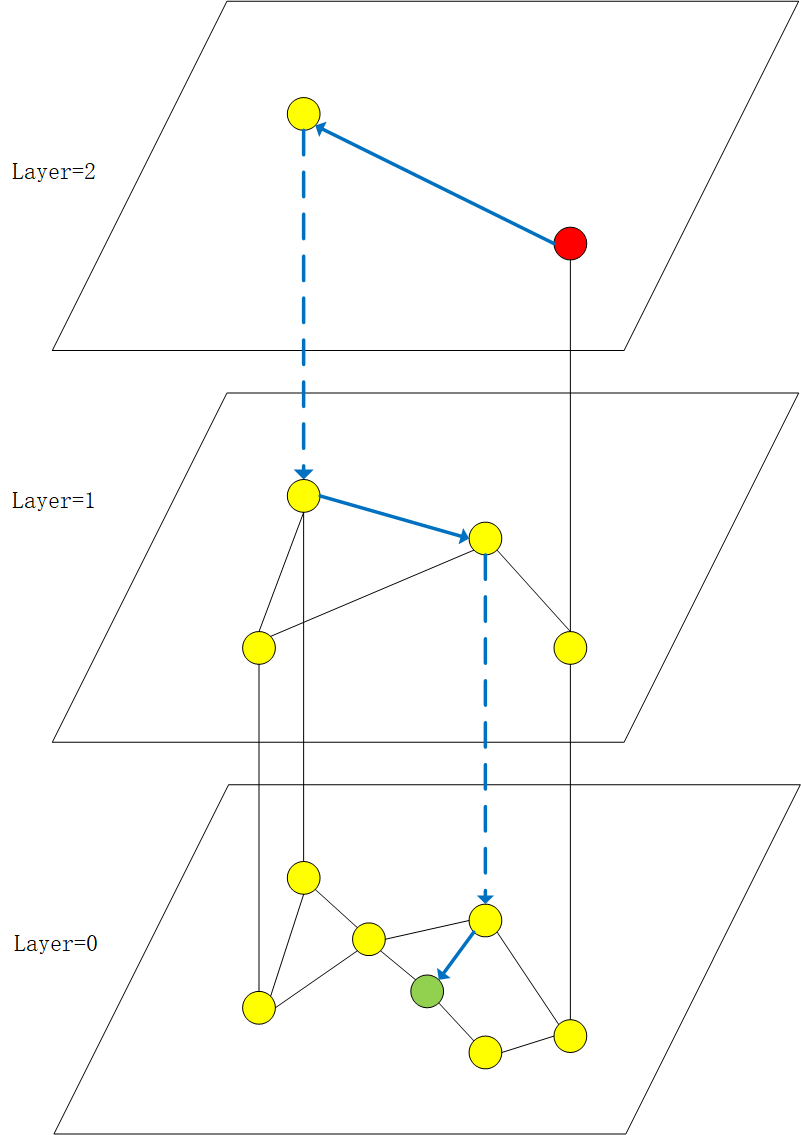
In the process of constructing the graph, each node will pre-calculate its degree, which is the highest level it will appear in the graph. If a node degree is 1, then it will appear in the layers of 0 and 1. And the 0th layer will have all the data, and the distribution of the data is that the higher the number of layers, the less the data, the greater the distance between nodes, so the search will be very fast and can be reduced the number of nodes that need to be traversed when searching.
When searching, it will enter from the entry point of the highest layer, and then use the greedy algorithm to find the local nearest neighbors between the layers to jump to the next layer, repeat this process to reach the 0th layer, and start the real search at the 0th layer. When searching, maintain a heap to store the nearest node, start searching all its neighboring points at the entry point of the 0th layer and determine whether to insert into the heap, and record the node closest to the query point among all neighboring points as the next starting point. Repeat the above process until the query results meet the conditions to end the query. As shown by the red dot and blue line in above figure , the red dot represents the entry point of the graph, the search starts from the red dot, the blue solid line represents the local nearest neighbor between the layers, and the blue dotted line represents the passing between layers. Jump into the next layer and repeat this process, and find the green point on the 0th layer to indicate that a search is completed.
For the data insertion process, when constructing the adjacency relationship of a certain node, it is also carried out layer by layer. For example, the degree of a certain node is 1, so that the node will only appear in the 0th and 1st layers, and only need to construct the adjacency relationship of this point in these two layers. When inserting, it will first enter the graph from the entry point of the highest level. As shown in the figure, starting from the red dot of the highest level, after finding its local closest point through the greedy algorithm, this point enters the first level and builds it on the first level. After the adjacency relationship, the same greedy algorithm finds the local nearest neighbor and then enters the 0th layer to start building the adjacency relationship.
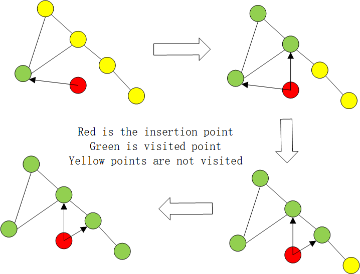
When constructing adjacency relationships at a certain level, a list of candidate points and a list of results, and a list of visited nodes are maintained to mark visited points to reduce repeated searches. The candidate point list records all possible candidate points, and the result list saves all adjacent points of the insertion point. The candidate point list records the visited points, and searches all its neighboring points from the entry point to see if these nodes have been visited. If they have not been visited and these nodes are closer, they will be inserted into the candidate point list. These closer points are inserted into the result list, and then the nearest node is found from the candidate point list to traverse all the neighboring points again, and the above process is repeated until the candidate point list is empty and the traversal ends, and the nodes that meet the conditions in the process will be saved to the result list and filter the nearest M nodes as the adjacent points of the insertion point. The process is shown in the figure below.
It can be seen that there will be a situation in real-time insertion and search, that is, when inserting, the HNSW graph will insert new nodes to expand, and the structure of the graph will be expanded. For example, in faiss, std::vector is used to store nodes. For adjacent nodes, once the expansion occurs, the internal storage structure of the previous vector will change. If there is a search at this time, the program will crash due to the search access to the invalid structure before the expansion, so a read-write lock will be added when searching and to protect the situation of inserting and searching at the same time.
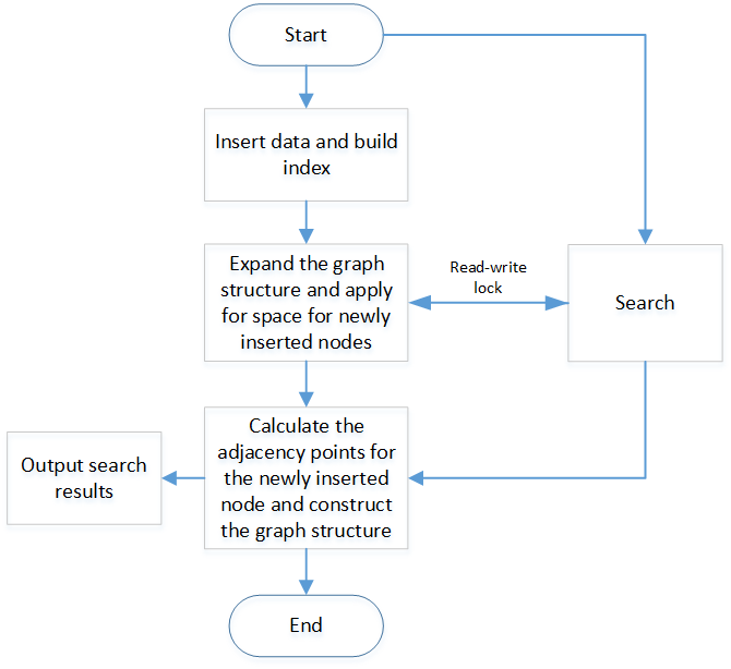
It can be seen that in the process of inserting and searching at the same time, the read-write lock only locks the expansion part of the graph structure, and the time-consuming part of this part is very small for building the index. The more time-consuming to build the index is for the newly inserted node calculates the part of the adjacent node, so the granularity of the entire read-write lock is small, which will not significantly affect the performance of the search.
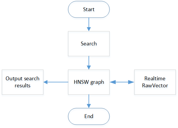
In addition, when querying, you will need a structure that can read the vector information of all nodes to calculate the distance. For example, a DistanceComputer is defined in faiss to access the vector information of all nodes, and VisitedTable is used to mark all the visited points, but when searching in real time , The query may encounter a new insertion point, and then use DistanceComputer to find the corresponding vector, but DistanceComputer is not dynamically expandable, unable to obtain the new insertion point information, so there will be out of bounds. The HNSW algorithm in vearch obtains all the vector information through RawVector, and RawVector can be inserted in real time, thus avoiding the situation of out of bounds. In addition, the design of the RawVector part can refer to the documentation of the RawVector part. The structure is shown in the figure below.