ICP
In this page, I'll discuss about why ICP (Iterative Closest Point) is deactivated by default (for RGB-D cameras). For some cases, enabling ICP will increase precision of the loop closure and the visual odometry. However for some other cases, it will add difficult detectable errors. The next sections show two cases: where ICP helps to give better transformations and where ICP doesn't help at all, even increase the error.
Note that for lidar, ICP works pretty well as the scans are generally very accurate: the field of view is large and range accuracy is very good. This article is about using ICP with RGB-D cameras, though same issues could happen with lidar in environments with low geometry (e.g., long corridor). For more camera versus lidar comparisons and ICP issues, see
- M. Labbé and F. Michaud, “RTAB-Map as an Open-Source Lidar and Visual SLAM Library for Large-Scale and Long-Term Online Operation,” in Journal of Field Robotics, vol. 36, no. 2, pp. 416–446, 2019.
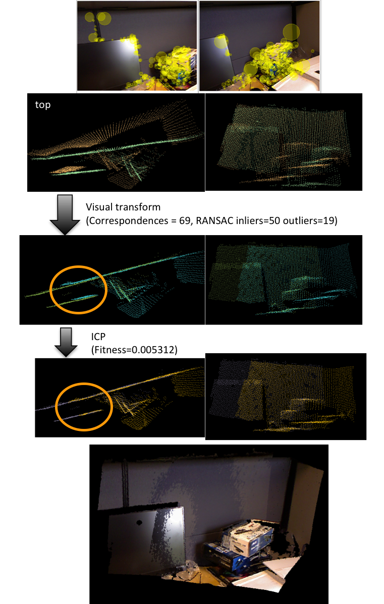
When a loop closure happens between two images, we compute the visual transformation using the corresponding visual words. When ICP is enabled, this transformation is used as a guess for the ICP algorithm. The image below shows this process.
- We have two corresponding images.
- We compute the visual transformation, the results show a little orientation error (see he first yellow circle) on the transformed clouds using this first guess.
- Using ICP, we refine this transformation using only geometric information. This orientation error is corrected (second yellow circle). In this case, ICP increases precision.
In this case, we do the same: we compute a visual transformation to find a guess for the ICP. The process is shown in the image below.
- We have two corresponding images.
- We compute the visual transformation, the results show that the clouds of the screen are correctly aligned (first yellow circle).
- Using ICP, we refine this transformation using only geometric information. However, here ICP decreases the precision. What happens is that ICP tries to match as many corresponding points as it can. Here the background behind the screen has more points that the screen itself on the two scans. ICP will then align the clouds to maximize the correspondences on the background. The screen is then misaligned (second yellow circle).
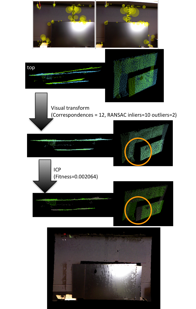
The ICP error on the second case is difficult to detect. For example, the euclidean fitness score (e.g., sum of squared distances from the source to the target) of the first case is 0.005312 and the second case is 0.002064. Generally, a fitness under 0.1 gives good results. However, in the second case, the fitness is even lower than in the first case, which makes this criterion not robust to detect such wrong cases. For this reason, ICP is disabled by default in RTAB-Map.
You can try the examples above on the corresponding PCD files:
| First case | Second case |
|---|---|
| old.pcd | old.pcd |
| new.pcd | new.pcd |
| icp.pcd | icp.pcd |
 $ pcl_viewer old.pcd guess.pcd //see transform using visual transformation guess only
 $ pcl_icp old.pcd guess.pcd
 $ pcl_viewer old.pcd guess.pcd //see transform with icp