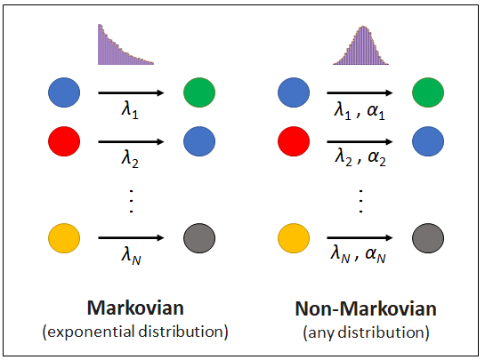
First, you need to install REGIR, or you can use the REGIR.py file provided in the repository:
- pip install REGIR
Then, you can run a non-Markovian simulation with the toy example below, or load an SBML model directly into REGIR (check out the REGIR/SBML folder for detailed instructions). Other examples, including the three biochemical systems described in the paper: Cell division, differentiation and RNA transcription, are provided in the /REGIR/Examples and /REGIR/Biochemical_applications folders.
import REGIR as gil

#Set the simulation parameters:
class param:
	Tend = 10		#Length of the simulation
	N_simulations = 20	#The simulation results should be averaged over many trials
	unit = 'h'		#Unit of time (used for plotting only)
	timepoints = 100	#Number of timepoints to record (used for plotting only)

r1 = 1
r2 = 4
r3 = 0.03
alpha1 = 20
alpha2 = 5

#Define the reaction chanels:
reaction1 = gil.Reaction_channel(param,rate=r1, shape_param=alpha1, distribution = 'Gamma')
reaction1.reactants = ['A']
reaction1.products = ['B']
reaction2 = gil.Reaction_channel(param,rate=r2, shape_param=alpha2, distribution = 'Weibull')
reaction2.reactants = ['B']
reaction2.products = ['C','A']
reaction3 = gil.Reaction_channel(param,rate=r3)
reaction3.reactants = ['A','B']
reaction3.products = []


#Define the initial population of reactants:
N_init = {'A':300,'B':0,'C':0}

#Initialize and run the Gillepsie simulation:
G_simul = gil.Gillespie_simulation(N_init,param)
G_simul.reaction_channel_list = [reaction1, reaction2, reaction3]
populations = G_simul.run_simulations(param.Tend, verbose = True)

#Plot the results:
G_simul.plot_inter_event_time_distribution()
G_simul.plot_populations()
The algorithm runs for a few seconds and output the following figures (note that you can disables all printing by passing the argument verbose = False when running the simulation):
The oscillations resulting from the markovian dynamics are clearly visible. If you check carefully, you will notice that the theoretical distributions do not match exactly the simulated distributions, even if you increase the number of simulations. This happens because the entities A and B are reactants of two reaction channels at the same time, and the theoretical distribution only represent the inter-event time distribution that the reaction channel would have if it was the only process interaction with that reactant. In practice, these kind of situations will occur frequently in non-Markovian systems, so do not worry if the simulated and theoretical distributions do not match exactly. The accuracy of REGIR was rigourously demonstrated in [1] (see the /REGIR/Benchmark folder).
With the current implementation, each available distribution are characterised by their rate and a shape parameter as follow:
  Exponential:
      - rate: 1/mean
      - shape parameter: None

  Normal:
      - rate: 1/mean
      - shape: std/mean

  LogNormal:
      - rate: 1/mean
      - shape: std/mean

  Gamma:
      - rate: 1/mean
      - shape: α >= 1 (https://en.wikipedia.org/wiki/Gamma_distribution)

  Weibull:
      - rate: 1/mean
      - shape: k >= 1 (https://en.wikipedia.org/wiki/Weibull_distribution)

  Cauchy:
      - rate: 1/median
      - shape: γ (https://en.wikipedia.org/wiki/Cauchy_distribution)
Keep in mind that non-Markovian simulations are only available for reaction channels with a single reactant, as the definition of inter-event time distribution is ambigious for channels with multiple reactants. If a channel is defined without or with more than one reactant, it will be considered as a Poisson process. Also, note that monotolically decreasing distributions, such as Weibull (k < 1), gamma (α < 1) or power laws, are not available in the current implementation of this repository, as these can be more elegantly and efficiently simulated with the Laplace Gillespie algorithm (LGA) [2].
Feel free to drop me an email if you have interest in me adding the Laplace Gillespie or any other relevant distributions to this implementation.
The REGIR framework offer countless possibilities and highly customizable models. However, with the current implementation, reactions propensities are always proportional to the number of reactant. For example, the reaction (A+B -> C) will have a propensity of a = A x B x r. In some models, you might want to implement more complex formula for the reaction propensities, (such as for example a = A x B x r / D, where D is a parameter that evolves with the system). To do so, you can directly modify the REGIR/compute_propensities function according to your need. Likewise, you might want to set up specific rejection rules if your reactants have some individual properties, and modify them appropriatly. To do so, first define your reactant properties in the REGIR/Reactant class, and then define your reaction specific rules in REGIR/ perform_reaction.
Feel free to email me if you are not sure how to do it, I will be happy to help !
[1] Pélissier, A, Phan, M, et al. "Practical and scalable simulations of non-Markovian stochastic processes". Submitted to Proceedings of the National Academy of Sciences (2022) [Preprint]
[2] Masuda, Naoki, and Luis EC Rocha. "A Gillespie algorithm for non-Markovian stochastic processes." Siam Review 60.1 (2018): 95-115.

