MRS Preprocessing and Basis Set Creation Using FID A and Analysis Using LCModel
If you’re looking at this page, then you probably have raw MRS data that you would like to process. This wiki will walk you through the different steps necessary to analyze your spectra and determine the concentrations of metabolites in your chosen brain area.
Where in MR imaging, water molecules are used to build an anatomical image of the brain, in MR spectroscopy a specific voxel is selected to collect a spectrum. This spectrum will show different peaks which largely come from protons in different chemical environments.
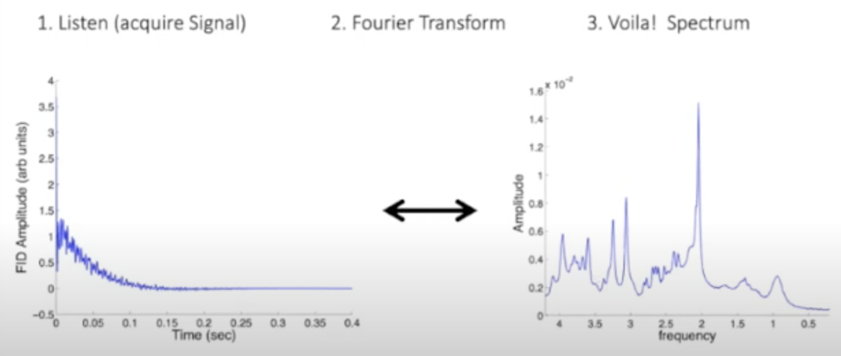
Just like you could decompose an audio recording of your favorite band into its different frequencies and determine which instruments were playing, in spectroscopy you acquire an electromagnetic signal and through a fourier transform over the time domain of the signal you get a spectrum of electromagnetic frequencies of different protons. This initial signal acquired is called the free induction decay signal, which through a fourier transformation will render a spectrum of electromagnetic frequencies.
 (Credit to Jamie Near)
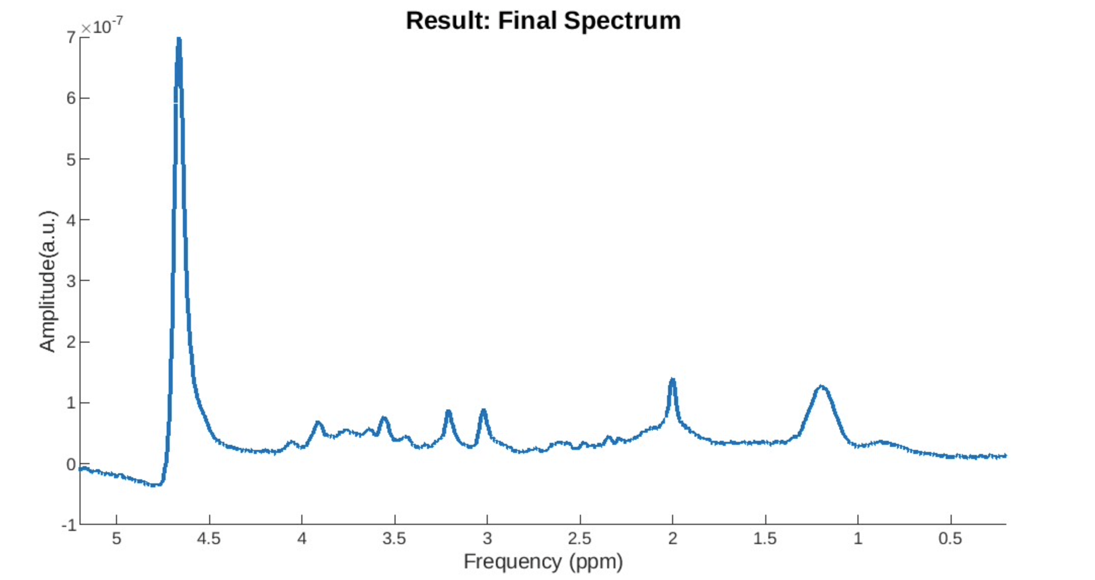
This MR spectrum is composed of signals from many different metabolites, and each of these metabolites has a highly unique and reproducible frequency distribution. This gives us a way to identify which metabolites are contributing to the signal and how much it is contributing. Where in a spectrum obtained from music the amplitude corresponds to the volume of an instrument, in MRS the amplitude is proportional to the concentration of the metabolite.
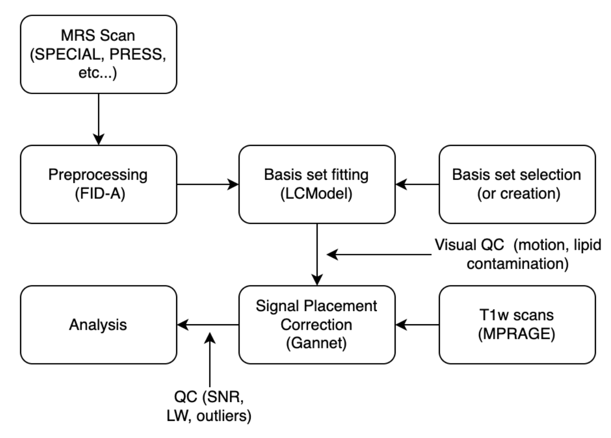
Broadly the steps necessary to process raw MRS data are the following:
- Acquiring the MRS scan (choosing the voxel of interest, performing system adjustments, combining and averaging many acquisitions into one usable FID signal).
- See for how to acquire: https://www.childrenshospital.org/sites/default/files/media_migration/f37f65af-bae3-49d5-8210-34be181f16bc.pdf
- See for different data structures output: https://bids-specification.readthedocs.io/en/bep022/modality-specific-files/magnetic-resonance-spectroscopy.html
- Preprocessing the raw data (correcting for motion drift, phase drift, eddy currents, etc… and outputting a clean spectrum).
- Basis-set fitting (get linear combination of metabolites that compose your spectrum, use water as peak reference to get absolute concentration of metabolite).
- Tissue correction (correct uncertain placement of voxel during scanning, get final estimated concentration of metabolites)
- Quality Control (Perform visual QC of voxel placement and spectra, remove outliers using SNR, Linewidth and Cramer-Rao Lower-Bounds)
- Analyze!
As such the following wiki will describe how to:
- Preprocess with FID-A
- Create or use an already existing basis set
- Fit your data using LCModel
- Implement tissue corrections to get your final metabolite concentrations
- Quality control voxel placement and spectra
The FID Appliance (FID-A) is an open-source software package developed by Dr. Jamie Near. FID-A can be used to simulate MRS experiments, design and analyze radiofrequency pulses, and process MRS data.
FID-A can be freely downloaded at http://www.github.com/CIC-methods/FID-A, wherein instructions to do so can be found as well. The FID-A software package consists of four toolboxes: the stimulation toolbox, the RF-pulse toolbox, the input-output toolbox, and the processing toolbox. Also, FID-A comes with a very detailed manual on its use, example run scripts, and example data. Before getting started, it’s also recommended to get a general understanding of how MRS functions and why all of the following steps are necessary - you can get a good overview of MRS in Jamie Near’s CIC lecture on the subject: https://www.youtube.com/watch?v=Pkv7legga6Y Notably, the steps below necessitate the download of MATLAB as well, as FID-A.
Before using FID-A, you need to organize your data appropriately as its autoprocessing scripts require folders to be organized in a very specific way.
First, if you are working from the CIC (which would be recommended), because you might need to re-organize the folder structure and because FID-A will be outputting many files, you will likely need to to copy all of your MRS data to your scratch. You can do this with the copy command:
cp “your/source/folder/”* “your/scratch/destination/folder/”Second, open MATLAB and add both FID-A and your data directory to your MATLAB path; this can be done in the MATLAB command lines using:
addpath(genpath(‘Full/path/to/FID_A/directory/’))Third, check how your folders are organized. FID-A will need a different file organization depending on whether you are running GE PRESS, SIEMENS PRESS or SIEMENS SPECIAL. FID-A needs to be run from a main folder, such that:
- main_folder > scan_ID > intermediate_folder > raw_file
The intermediate_folder and raw_file will change according to the scan sequence and scanner type. GE PRESS will have one scan per voxel as a P*.7 file. We recommend that you organize your folders such that you have a main folder containing your scan_ID folder, your voxel ID subfolder (e.g. acc, caudate, dlpfc) containing your P*.7 file.
- main_folder > subject/scan_ID > voxel_ID > P*.7
SIEMENS PRESS and SIEMENS SPECIAL will have the same organization only each scan ID will contain two (and only two!) folders called ID and ID_w, which each contain their respective water suppressed and water unsuppressed scans:
- main_folder > subject/scan_ID > ID & ID_w > water_supressed & water_unsuppressed
Your folder will likely not be organized this way naturally. It will likely be organized either with scan_ID inside an additional separate subject folder which contains all scans for that subject, and/or with no intermediary ID & ID_w folder.
- If your folders are organized correctly, move onto the next step.
- If your folders do not have an intermediary voxel_ID, ID or ID_w folder, you should write a bash script that puts the water suppressed file and water unsuppressed file inside their newly created ID and ID_w folders.
Generally, once navigating to the path within which the desired P-file is located, a single P*.7 file can be preprocessed in FID-A using the 'run_pressproc_GEauto.m' script by running:
[out,outw] = run_pressproc_GEauto('P*.7').Note that * would be replaced by the actual P-file name (e.g. P11776.7). This generates 'out' and 'out_w' in your workspace, which can be viewed by:
op_plotspec(out)and:
op_plotspec(out_w)'Out' and 'out_w' are outputs of 'run_pressproc_GEauto'; 'out' is the fully processed water suppressed data, while 'out_w' is the fully processed water unsuppressed data. Notably, for GE P-file data, the raw data for both water suppressed and water unsuppressed acquisitions are contained within the same P-file. Also, in the directory within which your P-file exists, two other new files are created: P*.7_lcm and P*.7_w_lcm, representing water suppressed and unsuppressed data, respectively. Notably, these files are in LCModel raw format and will be used below for LCModel analyses. Finally, after running 'run_pressproc_GEauto', a folder called 'report' will be generated, which contains an html file outlining the results of each processing step.
- If the steps above are not working for you, check the value for 'rdbm_rev_num' that appears in your workspace. You can determine this by putting a stopper on 'GELoad.m' found in 'inputOutput/gannetTools' after 'switch num2str(rdbm_rev_num)'. Ensure that the value that you are getting for 'rdbm_rev_num' (e.g. 20.0060) is captured within the 'GELoad.m' script as a 'case'.
- If your spectra look inverted, it may be related to a phase shift. This issue can be explored further and potentially addressed by using 'op_autophase', 'op_alignAllScans_fd', and/or 'op_removeWater'.
The data organization for preprocessing SIEMENS SPECIAL data using FID-A is similar to that of SIEMENS PRESS data detailed above. There are two raw .dat files. We organize these into two folders named as 'something' and 'something_w' (e.g. 'special' and 'special_w'). Next, we use the 'run_specialproc_auto.m'. To run one subject with the folder names detailed above, we would navigate to the directory within which the folders exist and run:
run_specialproc_auto('special')This generates a 'report' folder and a water-suppressed data file named 'special_lcm' within the 'special' directory, as well as a water-unsuppressed data file named 'special_w_lcm' within the 'special_w' directory. These new data files are ready for analysis by LCModel.
The steps here are generally similar to those detailed above for GE PRESS data. However, there are two notable differences. First, SIEMENS MRS data in the twix format has two .dat files (one water-suppressed and one water-unsuppressed), in contrast to GE MRS data, which had one P-file. Second, the other major difference from above will be the use of run_pressproc_auto.m as the .m file. Unlike above, here, the name of the folder containing the water-suppressed .dat file ('test' from the above example) is specified:
run_pressproc_auto.m('test')As above, this will generate a 'report' folder, and water-suppressed and water-unsuppressed data files. The 'report' folder and the water-suppressed data file will both be within the 'test' folder, whereas the water-unsuppressed data file will be within the 'test_w' folder. These data files can be imported directly into LCModel for analysis.
To run on several subjects you can use the same script as the SPECIAL protocol, only you will have to replace:
run_pressproc_auto.m('test')with
run_pressproc_auto.m('special')To run Matlab in batch there are two solutions:
- Create a main matlab file that processes one individual scan and then creates a separate bash script that calls it (recommended so you can use Qbatch).
Matlab Script:
function [MRS] = matthew_&_lani_preprocess(mrs_file)
    filelist = dir(mrs_file);
    %tests if you have the appropriate amount of files in your folder
    if length(filelist) != 4
        do nothing
    else
        [out,out_w]=run_specialproc_auto("special");
    end
Bash Script:
#create job list to run FID-A with Qbatch. Don't forget to load modules and execute from the right folder
dirs=`ls -d /data/scratch2/MatthewM/MRS/MRS_Data/HR/*`
for a in $dirs; do
	b in a; do
		echo matlab -nodisplay -r '"'"FID-A_Preprocess(""'"$(basename $b)"'"");exit"'"'
	done > joblist_FID-A
done
Run Qbatch:
qbatch -w 3:00:00 joblist_FID-A- Create a main matlab file that moves through all your files. You can find examples of this for:
a) GE PRESS:
- /data/chamal/projects/erics/erics_mrs_scripts/Preprocessing_GE_PRESS.m
b) Siemens SPECIAL:
- /data/chamal/projects/Matthew_M/MRS/MRS_Scripts/Fid-A-Modified/Matthew_scripts_mrs/matthew_lani_preproc_script.m
Full-width at half maximum and signal-to-noise ratio are two measures of spectral quality. These indices can be collected immediately after running 'run_pressproc_GEauto.m', since the 'out' and 'out_w' variables will already be in the workspace. However, if you forget to collect these measures for a particular dataset and you no longer have 'out' and 'out_w' in your workspace, you can bring them back into your workspace by loading in the 'P*.7_lcm' files through:
out=io_readlcmraw('P33792.7_lcm','dat');Linewidth and SNR can be extracted by running [lw,snr]=run_getLWandSNR(out). If you wish to collect these variables individually, you can do so as well by running:
SNR=op_getSNR(out); orLW=op_getLW(out);Choosing the right basis set is a major aspect of spectral quantification and can significantly change the metabolite concentrations you obtain. You have the choice between (1) simulating metabolites and creating your own basis with LCModel or (2) re-using one of those created by Jamie Near given you are using the same parameters.
To simulate a basis set to be used within LCModel analysis, the steps are as follows (using 'Lac', representing lactate, as an example). First, the metabolite is stimulated by running:
out=run_simPressShaped_fast('Lac')Next, we adjust it to ensure its compatibility with LCModel by running:
outmove=op_movef0(out,(4.65-2.3)*127)Finally, we write it back (to our working directory) as a .RAW file by running:
[~]=io_writelcmraw(outmove,'Lac.RAW','Lac')A script to do this for several metabolites at a time can be found locally at:
- /data/chamal/projects/erics/erics_mrs_scripts/basis_set_sim_GE.m
For this script, prepare an excel file listing the metabolites that you want simulated. When you run this script, you are prompted to select a file; all the metabolites in your file are then simulated, prepared for LCModel, and written back to your working directory as .RAW files.
- The refocusing pulse waveform 'GEref.pta' needs to be added and referenced appropriately in INPUT PARAMETERS in 'run_simPressShaped_fast.m'.
- If a 137 degree flip angle is used for data acquisition, appropriate alterations are necessitated in 'io_loadRFwaveform.m' to adjust for this. In speaking to Dr. Near about this, he has indicated that he will add the modified version of 'io_loadRFwaveform.m' to the repository. Thus, modification may not be necessary but utilizing the proper version of this .m is.
- In 'run_simPressShaped_fast.m', the values of the following INPUT PARAMETERS should be adjusted: refTp (duration of refocusing pulses), Npts (number of spectral points), sw (spectral width), Bfield (field strength), lw (linewidth), thkX and thkY (slide thicknesses of refocusing pulse), fovX and fovY (size of FOV), nX and nY (number of grid points to simulate), tau1 and 2 (TE for first and second spin echo), and refPhCyc1 and 2 (phase cycling steps for 1st and 2nd refocusing pulse).
- In 'run_simPressShaped_fast.m', the line:
refRF=io_loadRFwaveform(refocWaveform,'ref',0)was changed to:
refRF=io_loadRFwaveform(refocWaveform,137,0)- Ensure that you have the following MATLAB toolboxes: statistics and machine learning toolbox, parallel computing toolbox, signal processing toolbox, and curve fitting toolbox.
- A reference peak needs to be provided. Notably, Dr. Near has generated a reference peak spin system called "Ref0ppm" and uploaded it into the FID-A repository on GitHub. So, load spinSystems.mat OR load Ref0ppm. Then, run your simulation program using "Ref0ppm" as the specified metabolite and it will do the simulation for that peak. Finally, once it is simulated, the reference peak can be added to all of the other simulated peaks using (for example in the case of glutamate):
simGlu=op_addScans(simGlu,simRef)These steps are very similar to those detailed above for GE PRESS data. A script can be found locally at:
- /data/chamal/projects/eric/erics_mrs_scripts/basis_set_sim_siemens.m
For this script, prepare an excel file listing the metabolites that you want simulated. When you run this script, you are prompted to select a file; all the metabolites in your file are then simulated, prepared for LCModel, and written back to your working directory as .RAW files. Of note, as above, 'run_simPressShaped_siemens_fast.m' (a .m file made by altering 'run_simPress_Shaped_fast.m') should be edited accordingly. Particularly, the 'refocWaveform' needs to be a correct .pta file.
Important note for first-time users! If you are working remotely you will need to download LCModel yourself: http://www.lcmodel.com/lcm-test.shtml If working at the CIC, check that LCModel is available (if not check with Gabe you might have to switch desktops):
module availLoad module and launch:
module load lcmodel/20210527By now, you have simulated all of your metabolites, which exist as .RAW files in your working directory. Now it is time to turn them into a basis set to be used for analysis. For this, you can use LCModel's makebasis function. An example of the .in file you need to perform this task can be found at:
- /data/chamal/projects/eric/erics_mrs_scripts/makebasis.in
Adjust $seqpar and $nmall to your data. Of note, the dwell time (deltat) should match the dwell time of the simulated metabolites in MATLAB, not that of your data. Also, edit all of the 'filraw' lines in $nmeach and add/remove any stimulated metabolites that you have or do not have. Once your makebasis.in file is prepared, run the makebasis command in this way:
~/.lcmodel/bin/makebasis < makebasis.inMake sure you are in the top-level directory. This generates a .basis and a .ps file, the former of which will be used in the next step.
If you are using the CIC SIEMENS 3T MRI scanner on a SPECIAL sequence and a TE=8.5 ms, we recommend using Jamie Near’s basis set collected for this purpose.
You can find these basis-sets at:
- /data/chamal/projects/Matthew_M/MRS/special_basisset/
There are two basis sets you can use, the first models macromolecules as individual peaks while the second models them as a single basis function. We recommend asking Jamie Near what he thinks is best for your particular study, but largely the inclusion of many macromolecular components under the same basis set increases the degrees of freedom of LCModels analysis. This can lead on the one hand to more flexibility in the analysis when the macromolecular content and composition change (e.g., when pathological changes are present), but can also yield less accurate metabolite estimations without the application of certain constraints: https://onlinelibrary.wiley.com/doi/full/10.1002/mrm.27922
Now, we have preprocessed data and a basis set, and it's time to analyze our data. To do so through the terminal, we use .control files. Some examples of .control files can be found locally at: /data/chamal/projects/Matthew_M/MRS/MRS_Scripts/Fid-A-Modified/Matthew_scripts_mrs/md_runlcm_SPECIAL_3T_MMindiv.sh
Within a .control file, edit 'FILBAS', 'FILPS', 'FILTAB', 'FILH20', and 'FILRAW' to reflect the path to the .basis filename generated by the previous step, the output .ps filename, the output .table filename, the water-unsuppressed data filename, and the water-suppressed data filename, respectively. Also, other parameters need to be edited such as HZPPM, DELTAT, and NUNFIL, which represent the field strength in hz, the dwell time (1/spectralwidth), and the data points used, respectively. Finally, options such as water-scaling (dows) and eddy-current correction (DOECC) can be selected. To run LCModel using a .control file do:
~/.lcmodel/bin/lcmodel < controlfile.controlIf you want to run multiple subjects at a time, a .sh can be used:
dirs=`ls -d /path/to/mrs/data/*`
for a in $dirs; do
echo "Directory is " $a
/path/to/control/file /path/to/mrs/$(basename ${a}) special lcm unprocessed;
echo done ${a};
done
This script will produce multiple files among which you will find a .ps file in an LCM_out folder. You can view your spectra in the .ps file using a postscript viewer such as ghostview or evince. You can use ghostview after installing it:
gv *.psFinally you can collect all your LCM data into a .csv using a shell script:
#this script will take all of the analyzed data and jam it into a single CSV file.
dirs=`ls -d path/to/mrs/data/*`
subj='Subject ID,'

#put in the string 'Subject ID' in the first position:
echo "$subj" > mrs.csv

#Now append the first line in the output file, which is just the table column labels:
subj1=`echo $dirs | cut -d ' ' -f 1`
hdrs=`sed -n '1,1p' ${subj1}/special/lcm-out/unprocessed_lcm.csv`
sed -i "s|$| ${hdrs}|" mrs.csv

#Now add columns at the end for LW and SNR
sed -i 's/$/, Linewidth/' mrs.csv
sed -i 's/$/, SNR/' mrs.csv

#Now go through all of the subjects, and put in the subject ID,
#followed by the 2nd line of the CSV file for each subj.
for a in $dirs; do
    echo $(basename $a), >> mrs.csv;
    nums=`sed -n '2,2p' ${a}/special/lcm-out/unprocessed_lcm.csv`;
    echo "$(cat mrs.csv) $nums" > mrs.csv;
    lw=`grep 'FWHM' ${a}/special/lcm-out/unprocessed_lcm.table | cut -d '=' -f 2 | cut -d ' ' -f 2`
    SNR=`grep 'S/N' ${a}/special/lcm-out/unprocessed_lcm.table | cut -d '=' -f 3 | cut -d ' ' -f 3`
    echo "$(cat mrs.csv), ${lw}, ${SNR}" > mrs.csv
doneFrom your .csv file you will have collected 3 values:
- LCM metabolite output, an uncorrected estimation of the metabolites concentration in your voxel obtained through water scaling (mmol/L).
- A %SD or Cramer-Rao Lower-Bound. These are the estimated standard deviations expressed in percent of the estimated concentrations. These %SD estimates are only lower bounds, but they are still the most useful reliability indicators. As usual, you must multiply them by 2.0 to get rough 95% confidence intervals; i.e., the range that would contain the true value about 95% of the time. Ex: %SD > 50% indicates that the metabolite concentration could well range from zero to twice the estimated concentration.
- A relative estimation to creatine.
Once you have these three values you can quality control your values and spectra.
It is likely that you will eliminate most of the scans that do not pass a visual QC by using SNR and LW, nevertheless there are a few cases worth mentioning.
Eddy Current Issue: You can see a drop after the water peak and a subsequently elevated baseline.
Motion Drift: The spectrum does not have a stable baseline.
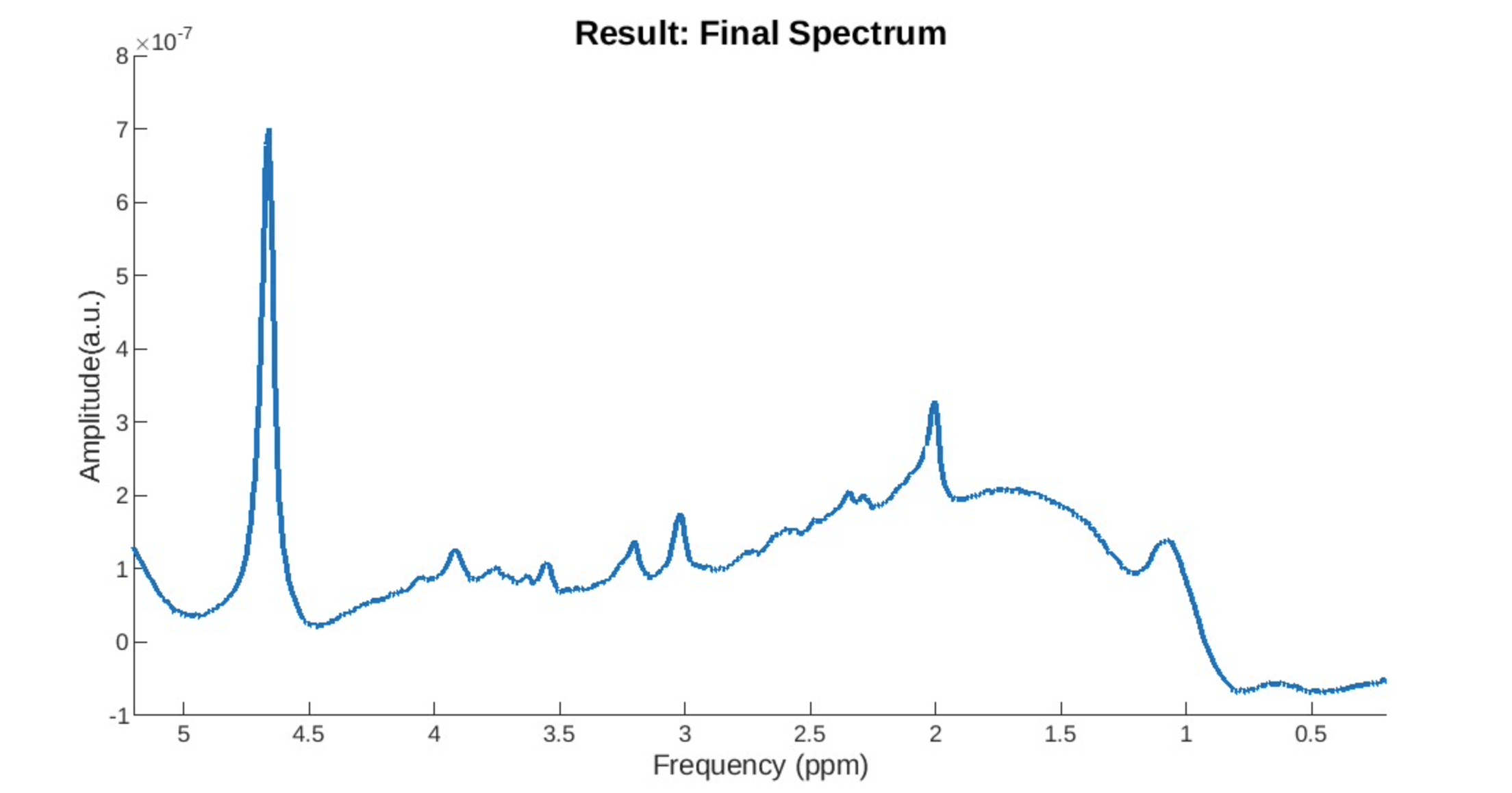
Lipid Contamination: Is harder to detect but is usually characterized by a lump.
The use of Cramer-Rao Lower-bounds is complex in MRS literature as these can vary widely from study to study. You can read about them in more depth here: https://pubmed.ncbi.nlm.nih.gov/25753153/ In our study we chose a Cramer-Rao Lower Bound of 25%. CRLBs are better used as a relative measure where if many metabolites have a high value relative to other metabolites or if one patient has many high metabolites compared to other patients, then it might be better to flag them. A better method is to calculate absolute bounds and apply them as weights when carrying out your analysis.
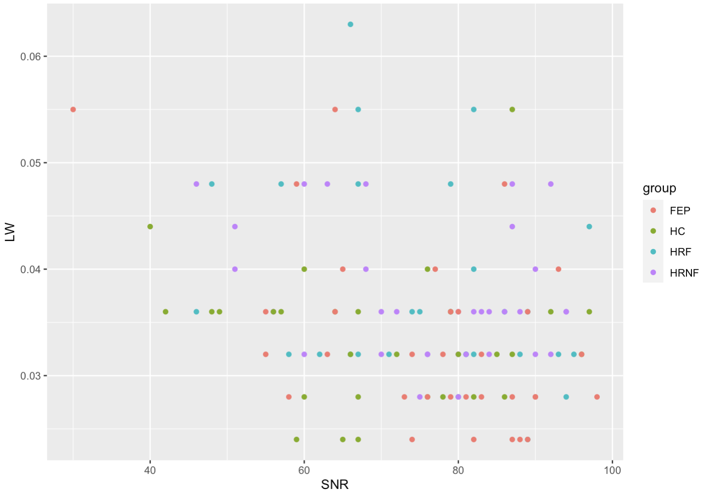
It’s a good idea to plot your SNR to LW to visualize who your outliers are in your study. In our study we eliminated outliers based on SNR (<20%) and eliminated all scans that had a LW superior to 0.08.
Because MRS voxels are chosen manually by the MR technician, and because physiologies of individuals vary, the voxels chosen obtained for one study can vary greatly. To correct this, we first look at where the voxel was placed by creating a label on the MRS voxel on a structural file. Then, because the concentrations of metabolites are different in the GM and WM, it is possible to estimate the absolute concentration of a metabolite in a region of interest by incorporating the GM/WM fraction in a voxel of interest into our calculation. For more details on how this is done you can read: https://www.researchgate.net/publication/330520594_Validation_of_in_vivo_MRS_measures_of_metabolite_concentrations_in_the_human_brain
In order to calculate the metabolite concentration in your voxel of interest you will have to first get the position of your voxel and overlap it with a structural file.
This can be done using Gannet through Matlab: https://doi.org/10.1002/jmri.24478
You can download Gannet here and follow instructions to set up all its dependencies (including SPM): https://github.com/markmikkelsen/Gannet
Before executing Gannet you will have to convert your structural file to .nii. You will have to decide which structural file you wish to use, but we recommend MP1RAGE scans for better contrast and estimations.
Depending on your OS and whether you have DCM files of MINC files you can use:
- dcm2niix
- mnc2nii
Note that Gannet only takes .nii files that have voxels saved in a 64-bit floating point format. If you are using the CIC’s pre-installed mnc2nii you will have to load mnc2nii and then run:
mnc2nii -nii -double path/to/.mnc path/to/nii/The best way to get Gannet to function in batch is to create a Matlab script that can carry out the fitting and segmentation of your spectra and structural file for one single file and then to write a .sh file that can iterate through your file and execute your matlab script in batch.
The main problem you will encounter here is getting your MRS data and your structural data to be in the same folder which is what Gannet requires if you want to run this in batch. Therefore you can either move the structural file to the same folder where your MRS data is in your scratch or fetch the structural data directly from the matlab script.
An example of a matlab script that runs Gannet over one file:
function [MRS] = Run_Gannet(mrs_file)
	data_dir_ = '/Users/username/Documents/my_project/data';
	filelist = dir(mrs_file);

	metab = {'S01_GABA_68_act.sdat'};
	metab = fullfile(data_dir, metab);
	% It is good practice to include the full path of files

	water = {'S01_GABA_68_ref.sdat'};
	water = fullfile(data_dir, water);

	anat = {'S01_T1_anat.nii'};
	anat = fullfile(data_dir, anat);

	MRS = GannetLoad(metab, water);
	MRS = GannetFit(MRS);
	MRS = GannetCoRegister(MRS, anat);
	MRS = GannetSegment(MRS);
	MRS = GannetQuantify(MRS);

	output_csv_file = fullfile(data_dir,"special/GM_WM.csv");
	table = struct2table(MRS.out.vox1.tissue);
	writetable(table,output_csv_file);
Running in batch:
#create job list for Qbatch run FID-A. Don't forget to load modules and execute from the right folder
dirs=`ls -d path/mrs/data/*`
for a in $dirs; do
b in a; do
echo matlab -nodisplay -r '"'"Run_Gannet(""'"$(basename $b)"'"");exit"'"'
done > joblist_FID-A
done
You can find an example of a matlab script that does not require importing the structural files to your scratch at:
- /data/chamal/projects/Matthew_M/MRS/MRS_Scripts/Gannet-main/Gannet-main-send/MRS_segmentation.m
You can then extract all of the MRS GM/WM fractions into a .csv file using the following .sh script:
#this script will take all of the analyzed data and jam it into a single CSV file>
dirs=`ls -d path/to/MRS/data/*`
subj='Subject ID,'

#put in the string 'Subject ID' in the first position:
echo "$subj" > Matt_HR_GM_WM.csv

#Now append the first line in the output file, which is just the table column l>
subj1=`echo $dirs | cut -d ' ' -f 1`
hdrs=`sed -n '1,1p' ${subj1}/special/GM_WM.csv`
sed -i "s|$| ${hdrs}|" Matt_HR_GM_WM.csv

#Now go through all of the subjects, and put in the subject ID,
#followed by the 2nd line of the CSV file for each subj.
for a in $dirs; do
    echo $(basename $a), >> Matt_HR_GM_WM.csv;
    nums=`sed -n '2,2p' ${a}/special/GM_WM.csv`;
    echo "$(cat Matt_HR_GM_WM.csv) $nums" > Matt_HR_GM_WM.csv;
doneIt is possible that some MRS voxels were too far out of the region of interest and should be eliminated entirely from the data set.
You can view your voxel while Gannet is running or in post processing by using the display function in the minc toolkit. To do so you will have to load the mink toolkit and the minc toolkit extras. Gannet will have output a mask of your VOI in the same folder as your MRS file in a .nii format which you can use as a label on your structural file. Then you can execute the following command:
Display -gray path/to/struct/.nii -label path/to/MRS/.niiExample of a voxel not on the DLPFC which was our region of interest:

We use the following correction factor to convert metabolite signal intensity measurements to absolute units of concentration as follows:
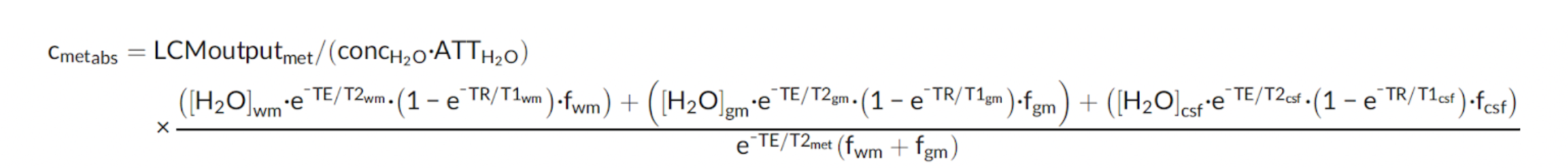
- Cmetabs: is the absolute concentration of a given metabolite
- LCMoutputmet: is the metabolite concentration in institutional units obtained from LCModel
- concH2O: is the LCmodel parameter specifying the tissue water concentration (= 35880 mmol/L)
- ATTH2O: is the LCmodel parameter specifying the attenuation of water due to relaxation and other effects (= 1.0 for SP, 0.7 for MP‐off, 0.43 for MP‐diff)
- [H2O]wm: is the assumed visible water concentration in WM (= 36100 mmol/L)
- [H2O]gm: is the assumed visible water concentration in GM (= 43300 mmol/L)
- [H2O]csf: is the assumed visible water concentration in CSF (= 53800 mmol/L)
- T2wm: is the assumed water T2 relaxation time of WM (= 79.2 ms)
- T2gm: is the assumed water T2 relaxation time of GM (= 110 ms)
- T2csf: is the assumed water T2 relaxation time of CSF (= 503 ms)
- T2met: is the T2 relaxation time of metabolite of interest based on literature values (see Table 1)
- T1wm: is the assumed water T1 relaxation time in WM (= 832 ms)
- T1gm: is the assumed water T1 relaxation time in GM (= 1331 ms)
- T1csf: is the assumed water T1 relaxation time in CSF (= 3817 ms)
- fwm: is the volume fraction of WM within the MRS voxel (determined from structural data) obtained through Gannet
- fgm: is the volume fraction of GM within the MRS voxel (determined from structural data) obtained through Gannet
- fcsf: is the volume fraction of CSF within the MRS voxel (determined from structural data) obtained through Gannet
- TE: is the echo time of the experiment (= 8.5 ms for SP and 68 ms for MP‐off and MP‐diff)
- TR: is the repetition time of the experiment (= 3200 ms)
This gives you the final absolute concentration of metabolites which can finally be used in conjunction with weights for analysis.