pydpiper: Running MAGeT.py on longitudinal data

Once you've run either twolevel_model_building.py or registration_chain.py, then the built-in MAGeT processing doesn't work properly (at least as of pydpiper 2.0.13) because MAGeT is run only within-subject. So, this tutorial documents how to run MAGeT for mouse brains afterwards.

MAGeTBrain works by performing non-linear deformation-based alignment using ANTS (Avants, Epstein, Grossman, & Gee, 2008) to map the high-resolution atlas to 25 template subjects, stratified across the data. All other subjects are then warped to the 25 templates, yielding 25 candidate segmentations per subject; final structure label was chosen by a voxel majority-voting procedure.

In order to run MAGeT, make a directory for your run.

Make a script for the run in the directory using a text editing tool like nano. Here is an example:

module load anaconda/5.0.1-python3 minc-toolkit/1.9.17  minc-stuffs/0.1.24^minc-toolkit-1.9.17 qbatch pydpiper/2.0.13
export PYDPIPER_CONFIG_FILE=/opt/quarantine/pydpiper/2.0.13/CIC-maget.cfg

MAGeT.py --verbose --pipeline-name=whateveryouwant \
--files /data/chamal/projects/elisa/maternal_infection/two_level_november/20171115_november_first_level/*_processed/*/resampled/*I_lsq6.mnc

You can always type MAGeT.py --help in your terminal to get options for the command. --verbose: will print jobs to screen

--pipeline-name: whatever name makes sense to you

--files: points it to the files to use as inputs. In this case, if you have a two-level model run, you can point it to the resampled lsq6 files in your first level. These are already registered to each other so which is required for MAGeT.py.

Now that you've saved your run script, you can run it in your run folder using bash. Keep that terminal window open, otherwise you will end your run.

Once your jobs have finished running, you'll want to perform quality control on your images. In your run directory you'll see a directory "pipeline-name_processed", in which you'll have a directory for each subject, in which there will be a voted.mnc file. This is your label file. You'll want to overlay each subject's voted.mnc file as a label on the input scan to ensure that the segmentation was successful. You'll want to do so using: Display 'input_scan.mnc' -label voted.mnc. Things to look out of are areas in which the scan was under segmented (the label does not cover the region completely) or oversegmented (the label bleeds outside of the ROI or outside the brain). These would be segmentation failures, or segmentations to be treated with caution.

Now you're ready to do statistics, so load:

module load R rstudio  minc-toolkit RMINC

In your R session, you'll want to load the following files as minc arrays or 3d volumes:

library(RMINC)
labelVol <- mincArray(mincGetVolume("/opt/quarantine/resources/Dorr_2008_Steadman_2013_Ullmann_2013_Richards_2011_Qiu_2016_Egan_2015_40micron/ex-vivo/DSURQE_40micron_labels.mnc"))
anatVol <- mincArray(mincGetVolume("/opt/quarantine/resources/Dorr_2008_Steadman_2013_Ullmann_2013_Richards_2011_Qiu_2016_Egan_2015_40micron/ex-vivo/DSURQE_40micron.mnc"))

These are going to be your label set (labelVol) and your atlas scan (anatVol).

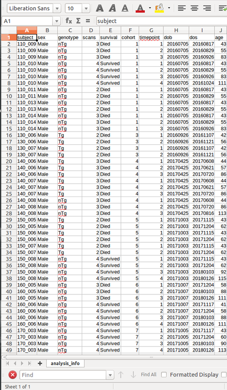
Next, load in your demographics files and set up your data frames so you are ready to do statistics. Below is an example of my csv:

Finally, you'll want to add a column to your dataframe with the absolute paths to your voted.mnc files, for example:

dataframe$label_file = paste0("path_to_voted.mnc")

voted.mncs may be found within [name-of-pipeline]_processed/*lsq6/ . In the more recent versions, there is a segmentation.csv that contains all relative paths to the segmentations from your run folder, which is quite easy to edit so as to have an ID column and the absolute paths instead. In older versions, to get the absolute paths, you had to do something like this:

dataframe$label_file=paste("path_to_pipeline", dataframe$scanid, "voted.mnc", sep="")
#makes a column with the absolute paths to all the labels

If you like, you can check that all of the paths point to files that actually exist with something like this:

# check that they exist
for (row in 1:nrow(dataframe)) {print(file.exists(toString(dataframe$label_file[1])))}

In order to turn your voted.mnc label files in to volumes, you will use the anatGetAll command. It will need your example atlas and label file as inputs. Here is an example:

dataframe$vols = anatGetAll(dataframe$label_file,
                                         defs = "/opt/quarantine/resources/Dorr_2008_Steadman_2013_Ullmann_2013_Richards_2011_Qiu_2016_Egan_2015_40micron/mappings/DSURQE_40micron_R_mapping.csv", method = "labels")

Now you have an orthogonal column of labeled volumes per subject. You can now perform a statistical test of interested (i.e. linear model) on all of the volumes you generated, and correct for multiple comparisons using the false discovery rate correction:

model=anatLm(~ fixed_effect_of_interest , data = dataframe, anat = dataframe$vols)
anatFDR(model)

Or maybe you have a longitudinal study design with missing data and want to run a linear mixed effects model!

In that case, the best choice may be to use a hierarchical model. First you'll need to load the definitions of the hierarchies:

hdefs <- makeMICeDefsHierachical("/opt/quarantine/resources/Dorr_2008_Steadman_2013_Ullmann_2013_Richards_2011_Qiu_2016_Egan_2015_40micron/mappings/DSURQE_40micron_R_mapping.csv", 
                                 "/opt/quarantine/resources/Allen_Brain/Allen_hierarchy_definitions.json")
# Then, create an array of the volumes labelled with the hierarchy
vols <- addVolumesToHierarchy(hdefs, dataframe$vols)

# Make model
# This one is a linear mixed effects model, but before choosing one, you should compare it to quadratic and cubic,
# consulting this page: https://github.com/CobraLab/documentation/wiki/Comparing-statistical-models-on-minc-files
model <- hanatLmer(~ genotype * age + sex + (1|subject) + (1|cohort), dataframe, vols)

# Correct for multiple comparisons and threshold
model = hanatLmerEstimateDF(model)
model.fdr = hanatFDR(model)
thresholds(model.fdr)

Great, so you got your stats! Time to visualize. If you want to look at your brain in nice, colorful slices, follow this:

# Make sure that the column name that is the third argument in hanatToVolume is a period (.), even though you might
# think it should be a dash (-). Current format as of 2018.11.14

stats <- hanatToVolume(model, labelVol, "tvalue.age")
# threshold (low and high) at the q-value you want to look at!
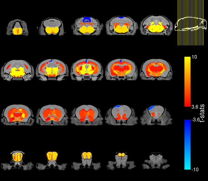
mincPlotSliceSeries(anatVol, stats, low=2.43, high=10, symmetric=T, legend="t-stats", begin=50, end=-50)

Does your image look something like this?

You can also consult this tutorial for more ways to edit and visualize your results! https://rawgit.com/Mouse-Imaging-Centre/RMINC/master/inst/documentation/hierarchiesTutorial.html