Investors are always evaluating the amount of risk they are willing to take for a certain expected return. Intuitively, the best investment maximizes the returns and minimizes the risks. Measuring risk and return, however, isn’t easy in the world of finance and economics. Capital Asset Pricing Model (CAPM), for example, measures an asset’s sensitivity to the market movements and provides the required rate of return for exposure to the systematic risk [1]. The required rate of return (RRR), a subjective measure, is the minimum return an investor seeks on an investment.

Fama-French Three-Factor Model

While still widely adopted, CAPM has several shortcomings [1], leading to the development of more comprehensive models. Fama-French Three-Factor Model, designed by Eugene Fama and Kenneth French, appends size risk and value risk to CAPM. The model, recognizing that investment in small-cap stocks, value stocks, and volatile stocks is riskier, calculates the required rate of return with the following formula [2]:

Where:

• RRR = required rate of return
• Rf = risk-free rate of return
• Rm = market portfolio return
• SMB = size premium
• HML = value premium

Let’s break down the formula a little bit more.

The risk-free rate of return is the theoretical return on investment (ROI) of an investment without any risks.

Since no investment is risk-free in the real world, government bills yield to maturity are usually used to measure the risk-free rate of return. The market portfolio return is the return of a portfolio consisting of all assets in the market.

The difference between the market returns and the risk-free rate of return is called the market risk premium and represents the extra returns an investor expects for exposure to market risks.

Small-Minus-Big (SMB) is excess returns of small-cap stocks over large-cap stocks.

High-Minus-Low (HML) is excess returns of value stock over growth stocks. β is the regression coefficient of asset returns for each factor and represents the mean change in returns for each unit of change in the predictor factor.

Factors

Professor Kenneth French publishes data for size premium, market premium, and value premium on his website. You can download the three factors daily records in CSV format from this page.

SMB and HML are the average excess return of three small and two value portfolios over large and growth portfolios. Market premium is the excess return of NYSE, NASDAQ, and AMEX firms over one-month Treasury bills.

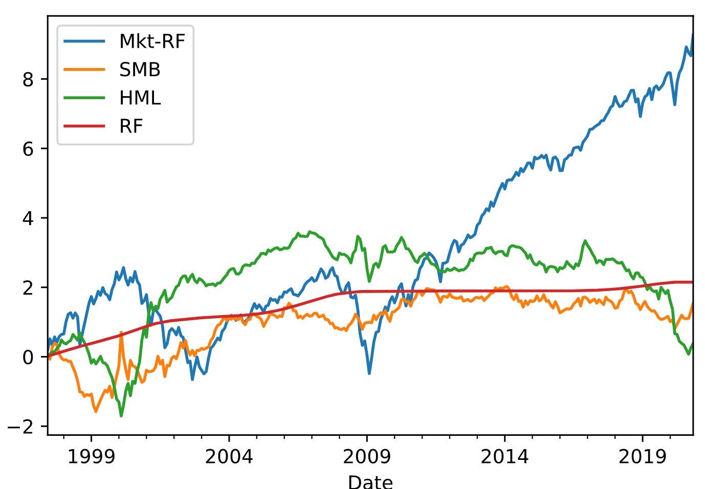
Let’s visualize the factors' historical records (note that we calculate the cumulative sum of factors for a better visual representation of the data):

factors = pd.read_csv("./data/factors.csv", index_col="Date")

# convert Date index to datetime object
factors.index= pd.to_datetime(factors.index, format="%Y%m%d")

# get monthly avg
factors = factors.resample('BM').mean()

factors_cum = factors.cumsum()
factors_cum.plot.line()

Asset Returns

We’ll use ETSY as an example for the rest of this article. Also, we get the ticker data using yfinance library.

import yfinance as yf

etsy = yf.Ticker("ETSY")
hist = etsy.history(period="max", auto_adjust=True, rounding=False)
price = hist[["Close"]]

# resample by latest monthly price
monthly_price = price.resample('BM').last()

# calculate monthly returns
monthly_returns = monthly_price.pct_change().dropna()

# calculate excess monthly returns
excess_returns = (monthly_returns['Close'] - factors['RF']).dropna()

# convert to dataframe
excess_returns = pd.DataFrame(data=excess_returns.values,
                              index=excess_returns.index,
                              columns=["Returns"])

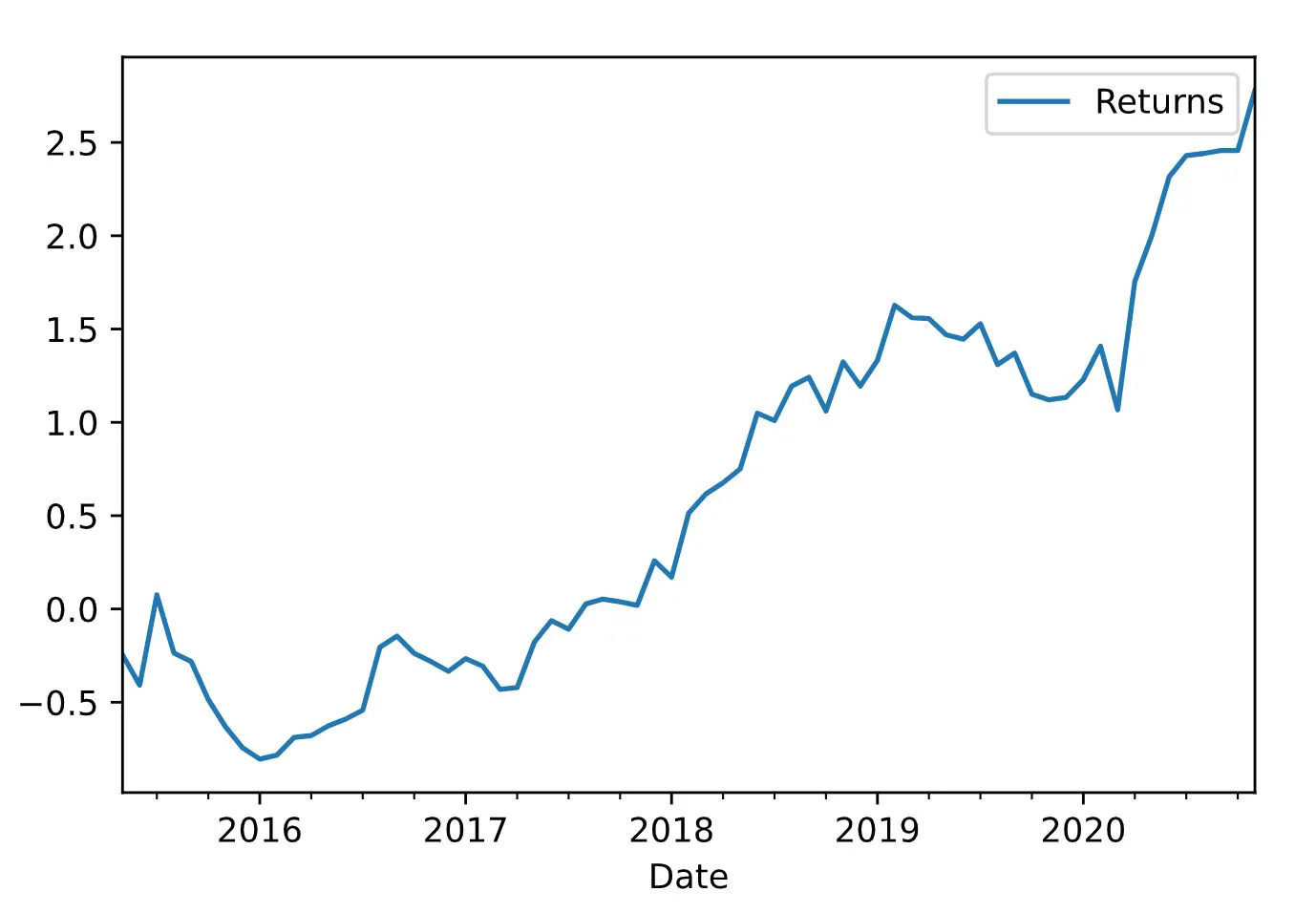
excess_returns_cum = excess_returns.cumsum()
excess_returns_cum.plot.line()

Beta

Since beta is the slope of the regression line, we can calculate it by running multiple OLS regressions–where factors are predictors and excess return is the dependent variable.

import statsmodels.api as sm

# join factors to returns dfs
data = factors.join(excess_returns).dropna()

y = data[["Returns"]] 
x = data[["Mkt-RF","SMB","HML"]]


ols = sm.OLS(y,x)

result = ols.fit()
betas = result.params
print(betas)

The result is:

Mkt-RF 0.344029 SMB 0.257253 HML -0.159444 

The Required Rate of Return

All the necessary ingredients to calculate the required rate of return using the Fama-French three-factor model are ready. We can now calculate the RRR.

latest_factors = factors.tail(1).to_dict('r')[0]

RRR = latest_factors["RF"]
RRR += betas["Mkt-RF"] * latest_factors["Mkt-RF"]
RRR += betas["SMB"] * latest_factors["SMB"]
RRR += betas["HML"] * latest_factors["HML"]

print(f"Required rate of return is: {RRR}")

Required rate of return is: 0.2462936811626845

---

[1] E.F. Fama and K.R. French, The Capital Asset Pricing Model: Theory and Evidence (2004), Journal of Economic Perspectives

[2] E.F. Fama and K.R. French, Common risk factors in the returns on stocks and bonds (1993), Journal of Financial Economics