Analysing Climatic Data with R Instat
R-Instat is designed as a general statistics package. All the calculations are made through the statistical system called R. In addition, there is a special climatic menu. Currently the methods are in the climatic menu are mainly designed for daily data. This guide uses an example of daily data for two stations in Guinea (Conakry) each of which was supplied with four elements. These data are in the R-Instat library and hence the examples in this guide can be followed by users who wish. The guide called “Preparing climatic data for analysis” covers the initial stages, up to the facilities for quality control of the data. This guide continues with the production of climatic summaries and graphs.
We gratefully acknowledge the permission of the Guinea Met Service for their permission to use their data in preparing this guide, and to allow their data to be added to the R-Instat library.
If you went through the first guide, then you will have your own copy of the file called guinea_r.rds.
- Open this file, either from where you saved it, or from the Instat library:
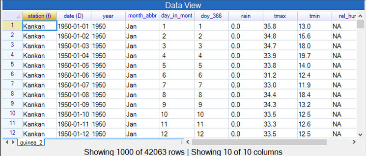
- (If from the Instat library use Open From Library > Load from Instat Collection > Browse > Climatic > Guinea and open the file called guinea_two_stations.RDS, Fig. 1
| Fig. 1 The Guinea data | Fig. 2 The column metadata |
|---|---|
 |
 |
 |
- On the toolbar press the icon with an i for information, see above.
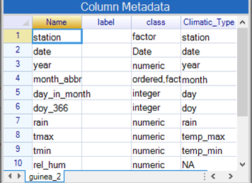
This shows the Column Metadata, Fig. 2. In the metadata, each row gives information about a variable, or column, in the actual data.
Check that the information includes the Climatic Type, i.e. that these data have been prepared for a climatic analysis. If not, then see Appendix 1.
- Press the same button again, or the toolbar button with the curly arrow, see above, to reset the windows to their default positions.
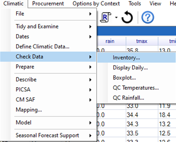
In the climatic menu, Fig. 3, the previous guide covered the use of the Dates, Define Climatic and the Check Data menus. We review an example of the inventory briefly, because it will help guide the climatic analyses later.
- Select Climatic > Check Data > Inventory, Fig. 3.
| Fig. 3 Climatic > Check Data > Inventory | Fig. 4 Plot for the rainfall |
|---|---|
 |
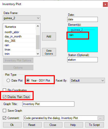 |
- Complete the dialogue as shown in Fig. 4.
- Press Ok to give the results shown in Fig. 5.
| Fig. 5 Seasonal patterns of the rainfall data |
|---|
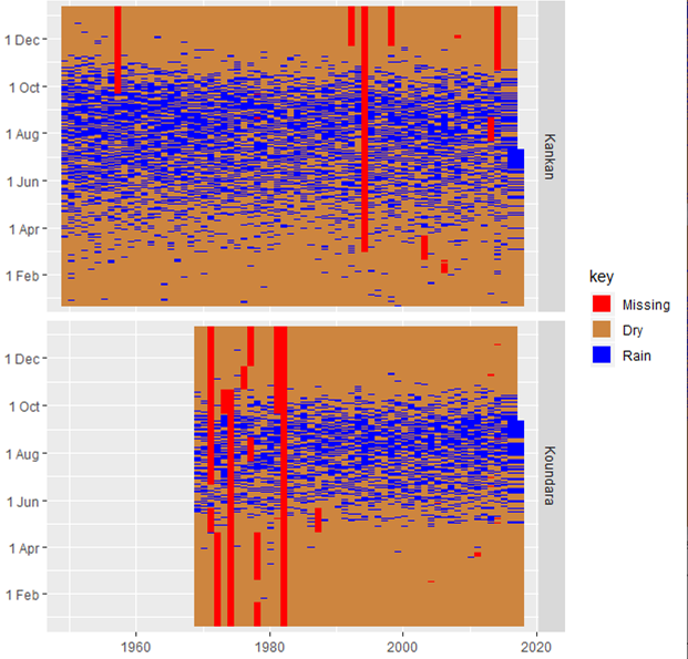 |
Our concern is the missing data, particularly in Kankan There are missing data in 4 or 5 years, that are in the dry period of the year and hence would not affect the annual totals particularly.
A second preliminary step is to facilitate calculating the number of rain days in the year. We show two ways this can be done.
- Use Climatic > Prepare > Transform
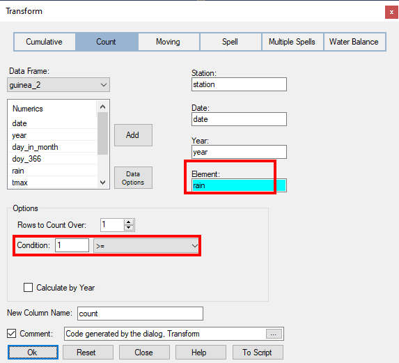
This dialogue should be set to the first button at the top, namely Count.
- Add the rainfall column, so the dialogue is as shown in Fig. 6.
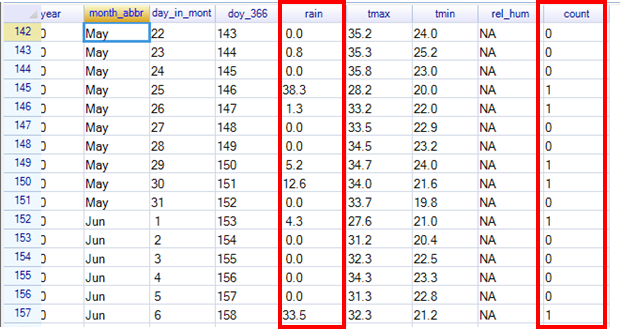
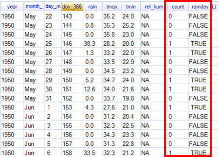
- Press Ok. This produces a new column which is 1 whenever there is a rain day, and zero otherwise, Fig. 7.
| Fig. 6 Dialogue for the Count of rain days | Fig. 7 The resulting variable |
|---|---|
 |
 |
In climatic analyses it is often useful to transform the data first, i.e. to add further columns to the data frame. Often, as here, you use the Climatic menu. After all it is designed to make climatic analyses as easy as possible.
Sometimes the transformation (or analysis) is not possible from the climatic menu. The task may still be possible using the more general facilities for the analysis. We illustrate here by producing the same column of rain days, using the general dialogues.
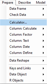
- Use Prepare > Calculator, Fig 8.
| Fig. 8 Prepare > Calculator | Fig. 9 Choosing the logical keyboard |
|---|---|
 |
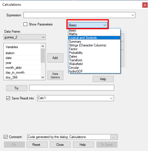 |
- In the calculator click on the pull-down, labelled Basic and choose the Logical keyboard, Fig. 9.
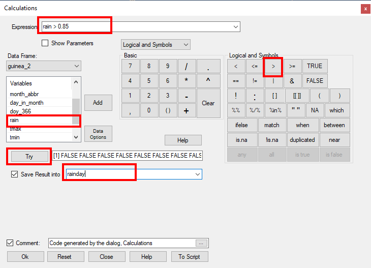
The calculator expands to show an additional keyboard, Fig. 10.
| Fig. 10 Completing the Calculate dialogue | Fig. 11 The new variable |
|---|---|
 |
 |
- In Fig. 10 choose the variable called rain. Double-click, or press on the Add button to put it into the expression.
- Press on > symbol and then on 0.85, Fig. 10. The expression is therefore rain > 0.85.
- Press the Try button, Fig. 10, to check you have a valid expression.
This should show FALSE for the first few rows of data, Fig. 10. This is because they are dry days, i.e. Rain is 0, and hence is less than 0.85mm.
If it said: “Command produced an error or no output to display.”, then you need to correct the expression.
- Save the result into a column called rainday, Fig, 10 and press Ok.
The result is shown in Fig. 11 for a few of the days.
- Scroll down in the data to confirm, Fig. 11, that when there is rain of more than 0.85mm the new column is TRUE. Otherwise it is FALSE. This is an example of a logical variable in R. It is used in just the same way as the column called count, because TRUE is interpreted as 1, and FALSE = 0.
So, as we show below, either of these variables can be used to give the total number of rain days. can total the number of TRUE values each year, to give the number of rain days.
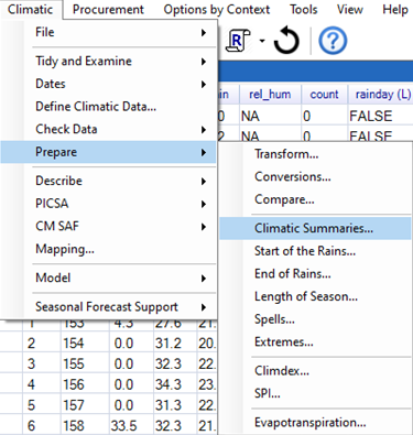
Now move back to the Climatic > Prepare menu in R-Instat
- Select Climatic > Prepare > Climatic Summaries, Fig. 12.
| Fig. 12 Climatic > Prepare menu | Fig. 13 Climatic Summaries |
|---|---|
 |
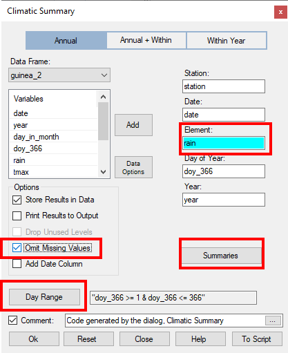 |
- Select the rain column as the element, Fig. 13.
- Click on the checkbox to Omit Missing Values. (Otherwise the summary is set to Missing whenever there is any missing day in the year.)
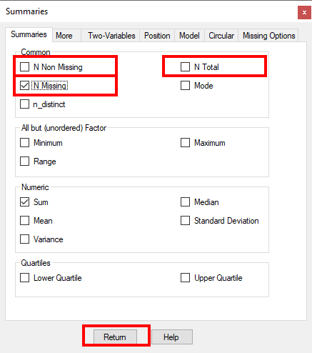
- Press the Summaries button to produce the sub-dialogue in Fig. 14.
- Untick N Non Missing and N Total, and tick N Missing, Fig. 14
| Fig. 14 Summaries sub-dialogue | Fig. 15 Day of Year sub-dialogue |
|---|---|
 |
 |
- Press on Return to go back to the main dialogue, Fig. 14.
If we wanted the rainfall totals for the whole year, then we could now click on Ok. But we choose them for the season, which we define as from March to October.
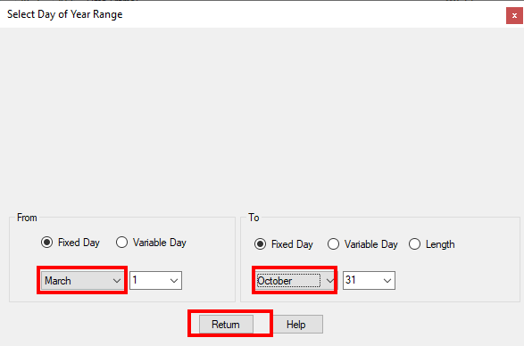
- So, click on Day Range in Fig. 13.
- Change the From month to March and the To month to October, Fig. 15.
- Press Return to go back to the main dialogue, Fig. 13; then press Ok.
This has produced a new data frame, with 116 rows, because there are 116 years of data in the 2 stations together.
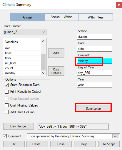
- Return to the last dialogue – use the icon on the toolbar, or use Climatic > Prepare > Climatic Summaries again.
- Change the element to rainday, Fig. 16.
- Press on the Summaries button, Fig. 16 and untick the checkbox to produce N Missing.
- Press Return on the sub-dialogue and then Ok.
| Fig. 16 Climatic summaries again | Fig. 17 Resulting summaries |
|---|---|
 |
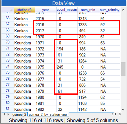 |
The results are in Fig. 17. For example, in 2016, Kankan had 1333mm total between March and October from 92 rainy days.
The early years at Koundara also have many missing values. There is an option in the Climatic Summaries dialogue to cope with this. But we illustrate here with another method.
- Use the Prepare > Calculator dialogue again. You can recall the last 10 items from the toolbar.
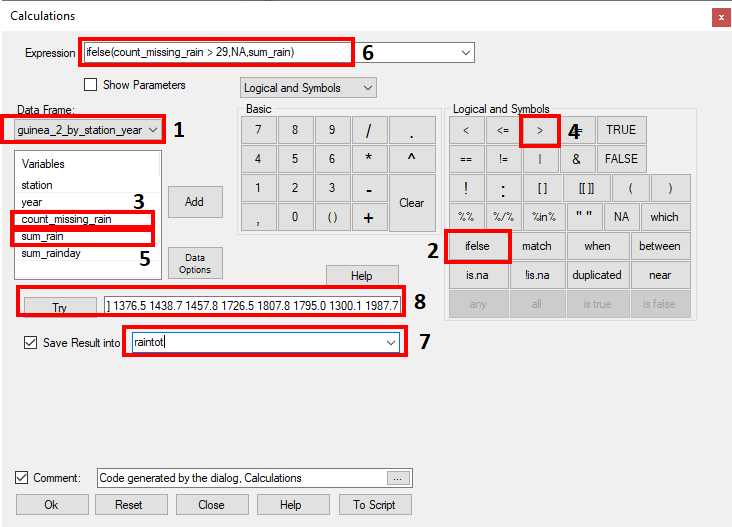
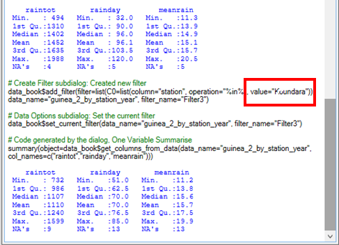
Complete the calculation as shown in Fig. 17. Then any year with more than 29 missing days will have the result set to missing.
This is not so easy, so numbers are included in Fig. 18 to provide the order, as follows:
- Step 1: Check you are on the correct data frame. It is guinea_2_by_station_year.
- Step 2: Press on the ifelse function.
- Step 3: Select the column called count_missing_rain.
- Step 4: Press on the “>” sign, and add 29 to the formula.
- Type then NA and then another .
- Step 5: Select the column called sum_Rain.
- Step 6: Check the formula is now ifelse(count_missing_Rain > 29 , NA , sum_Rain).
- Step 7: Rename the resulting column as raintot.
| Fig. 18 Setting summary data to missing | Fig.19 Resulting data |
|---|---|
 |
 |
- Step 8: Click on the Try button to check the command is giving results and not an error.
- Press Ok to produce a new column.
Now the same is done for the number of rain days.
- Get the dialogue back – use the icon on the toolbar.
- In the formula, point 6 in Fig. 18 change the variable sum_rain into sum_rainday. (Usually we suggest avoiding typing into this field, but it is tempting to just type the letters day here.)
- Change the name (Step 7) into rainday.
- Press Ok.
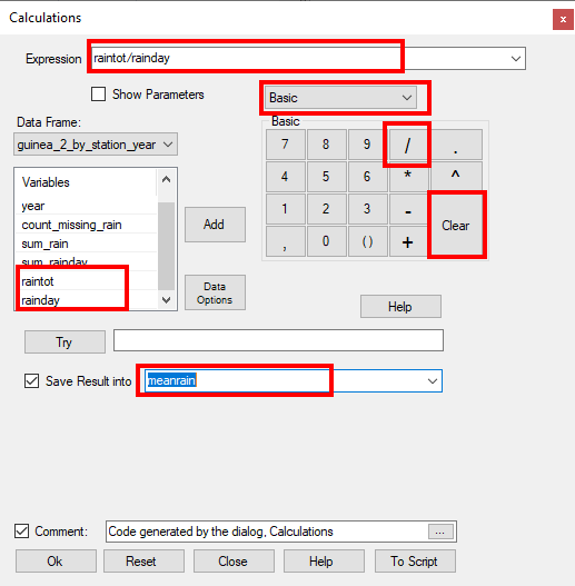
With the rainfall totals and the number of days, the mean rain per rain day can also easily be calculated.
- Get the last dialogue back (or use Prepare > Calculator again).
- Set the calculator back to Basic, Fig. 20.
- Press the Clear button
| Fig. 20 Calculate mean rain per rain day | Fig. 21 One Variable Summarise menu |
|---|---|
 |
 |
- Enter the formula raintot/rainday in Fig. 20 - no typing, just click.
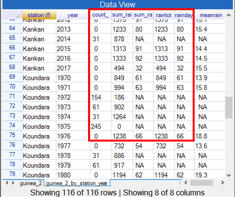
- Name the resulting column meanrain and press Ok. This produces the results on Fig. 19.
These summary data are processed in later sections of this guide.
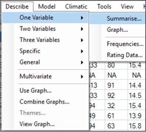
- For now, use Describe > One Variable > Summarise, Fig. 21, to get an initial idea of the columns produced.
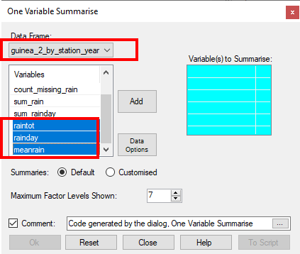
- Check that you are processing the correct data frame, i.e. the annual summary values.
- Select the 3 columns as shown in Fig. 22.
- Press Ok.
| Fig. 22 One Variable Summarise | Fig. 23 Results |
|---|---|
 |
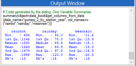 |
The results are shown in Fig. 23. For example 120 was the maximum number of rain days in the year.
These results are not actually very useful, because they treat the 2 stations together.
- Return to the same Summarise dialogue.
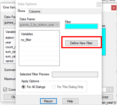
- Press on Data Options, see Fig. 24.
| Fig. 24 Data Options for a filter | Fig. 25 Filter for one station |
|---|---|
 |
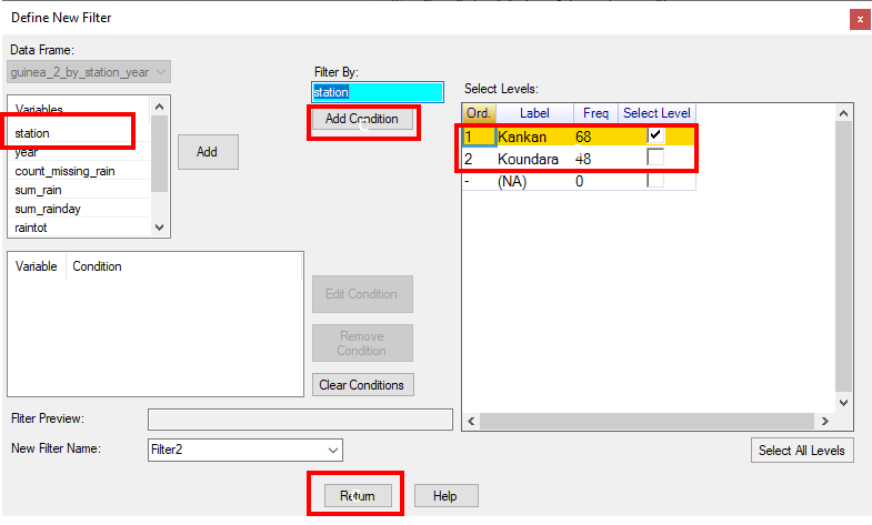 |
- Select the station column, Fig. 25
- The condition is correct to select just Kankan, so press on Add Condition.
- Then press Return to return to the sub-dialogue in Fig 24 again.
- Press Return again to return to the Summarise dialogue.
- Press Ok to get the results for just Kankan.
- Repeat the Data Options again, this time filtering for just Koundara in Fig. 25.
- Back on the main dialogue press Ok again to get the results for just Koundara, see Fig. 26
| Fig. 26 Results for each station |
|---|
 |
In this section you have taken daily data and produced some annual summaries. These were rainfall totals, but could equally have been other values, such as temperature means or extremes.
These summaries were put into a second data frame and were then analysed further.
The calculator was used to produce some further columns (variables) also at the annual level.
The analyses were for both stations together. The filtering facilities then permit results to be given for individual stations.
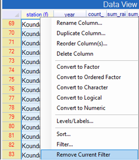
If you completed the analyses above, then a filter is in operation, Fig. 1, so just the data for Koundara are visible. In Fig. 1 the first row is in red, and this confirms a filter is being used.
- Right-click with the cursor in the name field, Fig. 1.
- Take the last option, to Remove Current Filter.
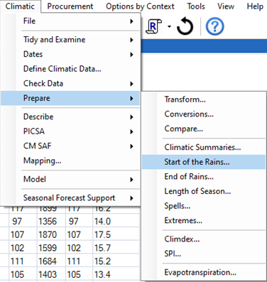
- Choose Climatic > Prepare > Start of the Rains, Fig. 2.
This is the menu item just below the Climatic Summaries used in the last section.
| Fig. 1 Removing the filter | Fig. 2 Choose Start of the rains |
|---|---|
 |
 |
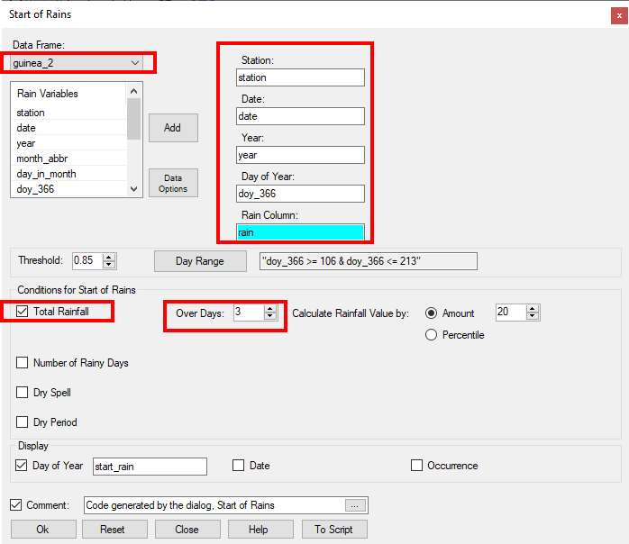
- In Fig. 3 check that the daily data **guinea_2 ** file is being used.
Note that the 5 fields from Station to the day of the year have filled automatically.
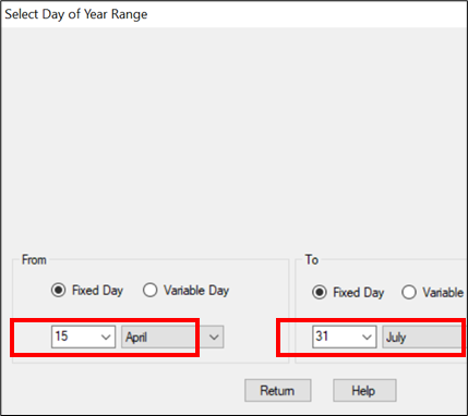
- Click on the Day Range, Fig. 3 to show the sub-dialogue, Fig. 4.
- In Fig. 4, change the From date to 15 April. That is the earliest date considered for planting.
- Change the To date to 31 July. We assume that no start by that date would then be too late.
- Press Return.
| Fig. 3 Start of the Rains | Fig. 4 Choose the earliest starting date |
|---|---|
 |
 |
- In Fig. 3 click on the Total Rainfall checkbox and change the 2 days to 3 days.
- Press Ok.
This adds a further column, called start, into the data frame with the annual data.
This may be termed a potential start date each year.
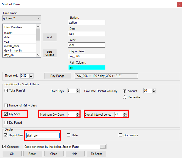
Now a second definition that also includes a dry spell.
- Return to the last dialogue.
- Click on the checkbox to add a dry-spell condition, Fig. 5
- Change the spell length to 7 days and the length of the period to 21 days.
- Name the resulting column as start_dry, Fig. 5.
- Press Ok.
| Fig. 5 Adding a dry spell condition | Fig. 6 Difference between start dates |
|---|---|
 |
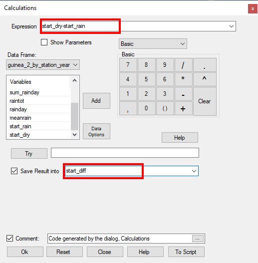 |
Now calculate the difference between these two columns
- Use the toolbar icon, or Prepare > Calculator, to get the R-Instat calculator
- In Fig. 6 the expression is start_dry – start.
- Call the resulting column start_diff.
- Press Ok. This adds a further column to the data. We interpret the result that when the column start_diff is zero i.e. the dry spell condition had no effect, then the first start date was ok. Otherwise, there was a dry spell of more than 7 days in the first 3 weeks (21 days) after planting, and hence replanting was needed.
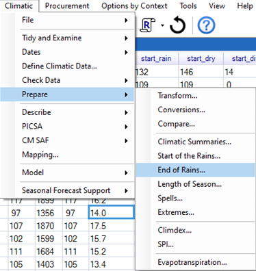
- Choose Climatic > Prepare > End of the Rains, Fig. 7.
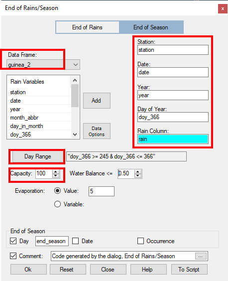
- In Fig. 8 confirm that the data frame is guinea_2, i.e. with the daily data. Hence that the controls on the right-hand side have been filled automatically.
- Press the Day Range button to give the sub-dialogue.
- Change the earliest date to 1 September. Press Return.
- Click on the End of the Season checkbox. Change the Capacity to 100mm.
- Press Ok.
| Fig. 7 Choose end of the rains | Fig. 8 End of the season |
|---|---|
 |
 |
This has used a simple water-balance model to give the date of the end of the season.
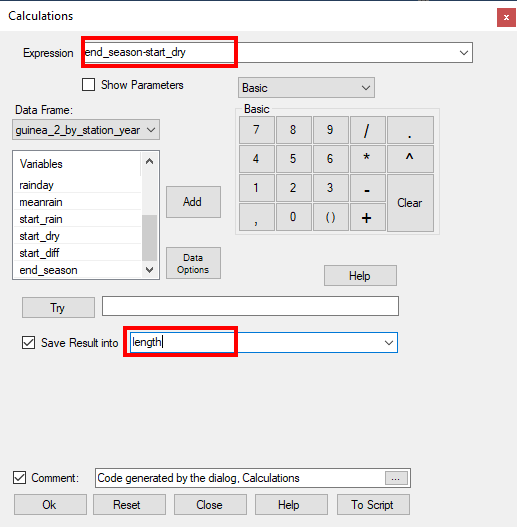
Now we subtract the start date from the end date, to give the length of the season.
- Use the toolbar icon to recall the Calculator, (or use Prepare > Calculator).
- In Fig. 9 the expression is end_season - start_dry.
- Call the resulting column length.
- Press Ok.
| Fig. 9 Calculate the season length | Fig. 10 Spell length menu |
|---|---|
 |
 |
Now calculate the length of the longest dry-spell in the season. This could be for a fixed set of months, e.g. July to September. Here we calculate the longest spell between the start and the end dates, and they are different each year.
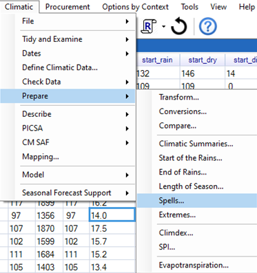
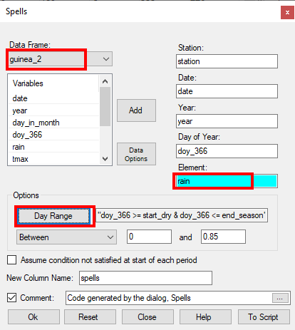
- Choose Climatic > Prepare > Spells, Fig. 10.
| Fig 11 Spell Lengths | Fig. 12 Choose day range |
|---|---|
 |
 |
- In the dialogue, check that the daily data – guinea_2 is being used.
- Add the rain column as the element, Fig. 11.
- Press the Day Range button, Fig. 11.
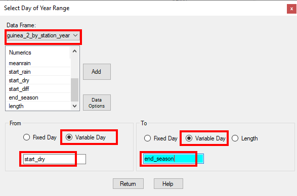
- In the sub-dialogue, on From click on Variable Day, Fig. 12.
- Check that this data frame has the summary data, i.e. guinea_2_by_station_year, Fig. 12.
- Choose start_dry as the starting column.
- In the To section, use Variable Day also and select the column called end_season.
- Press Return.
- Press Ok.
| Fig. 13 The summary data |
|---|
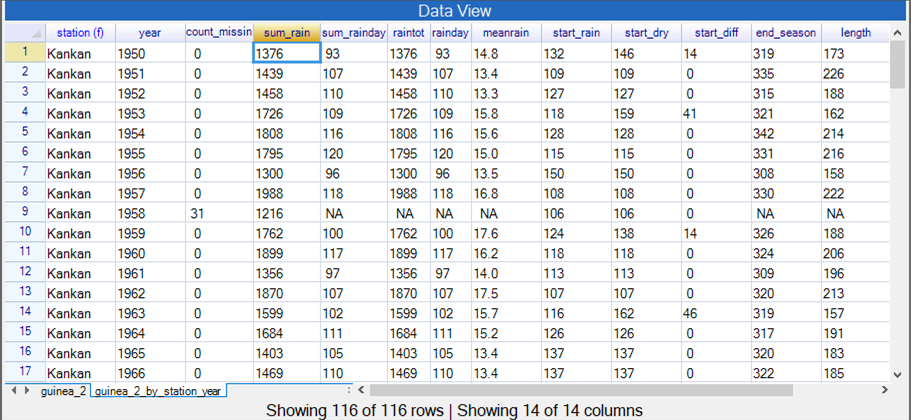 |
Fig. 13 shows that there are now many columns of data to examine further. For example, in Kankan in 1950:
- The total rainfall, from March to October was 1376mm
- This was from 93 rainy days and there were no missing values in this period
- The first start was on day 132, i.e. 11th May.
- The successful start was 2 weeks later, i.e. replanting was needed.
- The end date was day 319, i.e. 14 November
- Hence giving a season length of 173 days, almost 6 months.
- The longest dry spell within the season was 7 days.
The further analysis starts in the next section.
To complete this section, save the file.
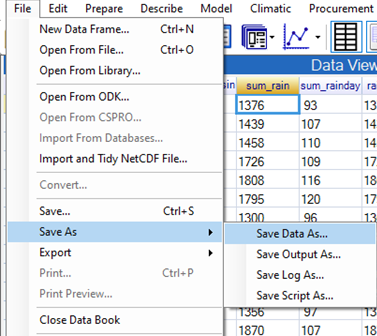
| Fig. 14 Save the data file | Fig. 15 Select a name |
|---|---|
 |
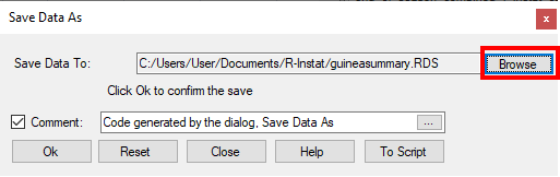 |
- Use File > Save As > Save Data As, Fig. 14.
- Press the Browse button, Fig. 15. In the subsequent dialogue choose a suitable directory and filename and click Save.
- You return to Fig. 15. Click Ok.
You may also use File > Export if you wish. But there is now a big difference between the exported and the saved file. Export is for a single data frame, while the Save is for the daily and the annual data together. So it is easy to resume the work on a later occasion.