Introductory Tutorial: Part 2 A Second Data Set
This tutorial guide follows on from Part 1 of the introductory tutorial. We recommend starting with Part 1, although this part is independent of the data and steps from Part 1.
This is daily climatic data from Dodoma in Tanzania, from 1935 to 2013. (Footnote: We are very grateful to the Tanzania Met Authority who have given permission for these data to be used for training purposes.)
-
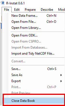
If the diamonds data are still in R-Instat then use File > Close Data Book, Fig. 16.
-
You will be asked if you are sure. Respond Yes.
| Fig. 16. Closing the previous data file | To start again |
|---|---|
 |
 |
-
Use File > Import from Library.... Take the option to Load from Instat Collection and then press Browse.
-
Choose Climatic and open Tanzania.
-
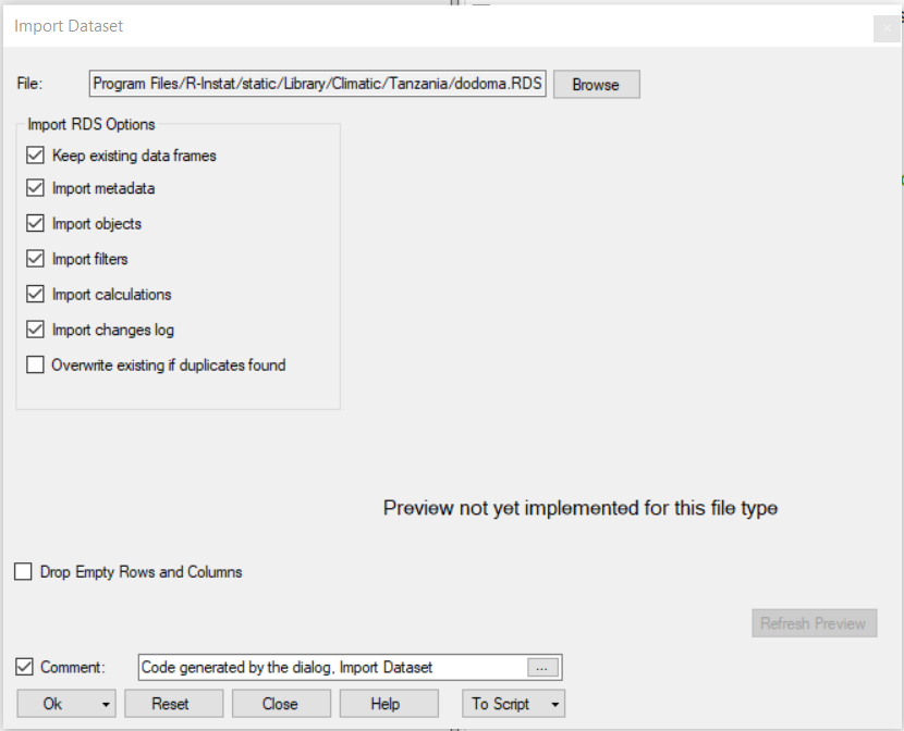
Open dodoma.RDS.
-
Click Ok to open in R-Instat, see Fig. 18.
OR
-
Use File > Import from Library. Take the option to Load from Instat Collection and then press Browse.
-
Choose Climatic and select the Excel file climatic_guide_datasets.
-
This Excel file has multiple sheets. Choose the one called dodoma, see Fig. 17
-
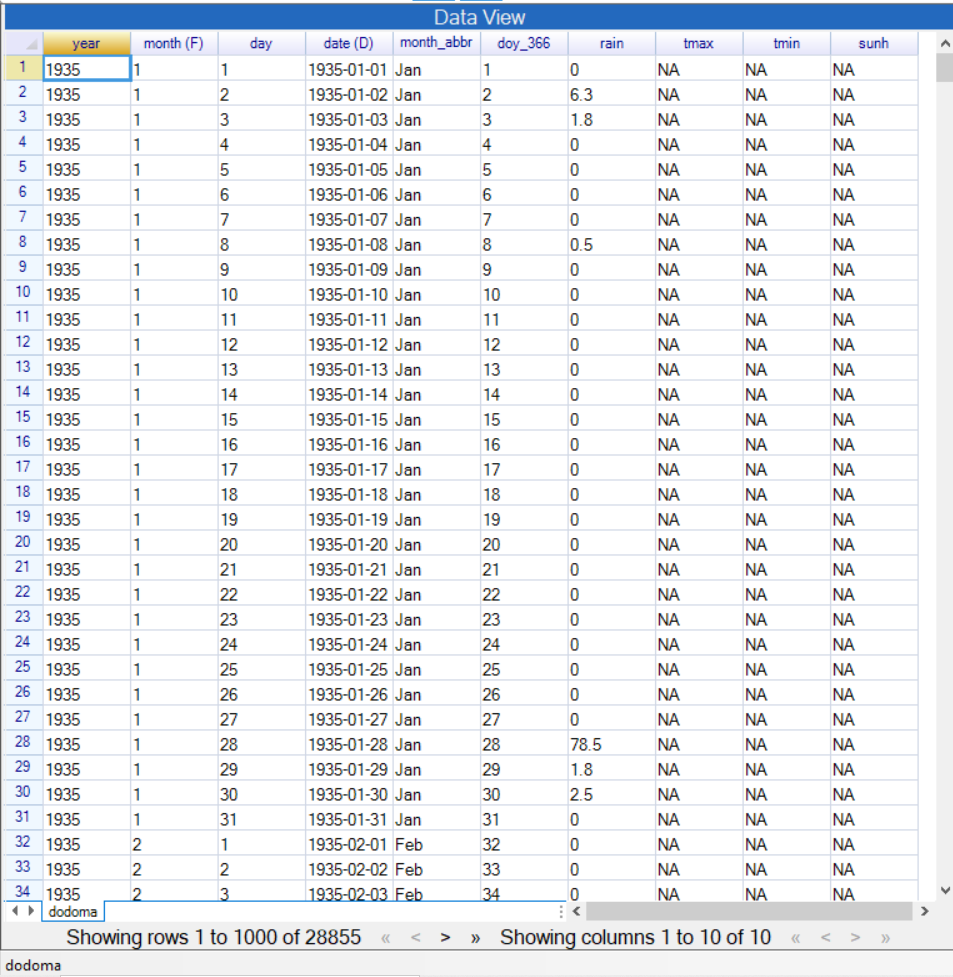
Press Ok. This opens the dataset see Fig. 18.
| Fig. 17 Opening the Dodoma sheet | Fig. 18 Dodoma Dataset |
|---|---|
 |
 |
An initial objective is to provide time series graphs for the annual mean temperatures, both maximum and minimum . The data are daily, and have first to be averaged to an annual level.
The first step is to change the Year column, which is numeric, into a category, or factor type of column.
-
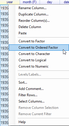
Go to the Year column and to the top (name) row. Right-Click, Fig. 19.
-
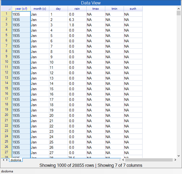
Click on Convert to Ordered Factor. See Fig.20 for the resulting data the year column now has O.F in brackets standing for ordered factor.
| Fig. 19. Convert to ordered factor | Fig. 20. The resulting data |
|---|---|
 |
 |
The daily data are now ready to be summarized to produce the yearly means.
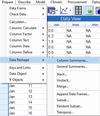
- Open the Prepare > Data Reshape > Column Summaries... dialogue, Fig 20.
| Fig. 20. Prepare > Data Reshape > Column Summaries... | Fig 21. Column Summaries Dialog |
|---|---|
 |
 |
-
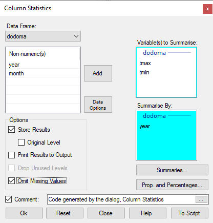
Complete the dialogue as shown in Fig. 19, i.e. tmin and tmax into the main receiver 'Variable(s) to Summarise:', year into the other receiver 'Summarise By:' , and the option ticked to Omit Missing Values.
-
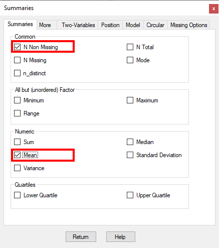
Then press the Summaries... button to move to the sub-dialogue, Fig. 21.
-
Complete the sub-dialogue as shown in Fig 21, i.e. with only two summaries for the N Non Missing and the Mean. Then press Return.
-
Press OK to produce the summaries, Fig. 22.
| Fig. 21. Summaries sub-dialogue | Fig. 22. With the resulting data |
|---|---|
 |
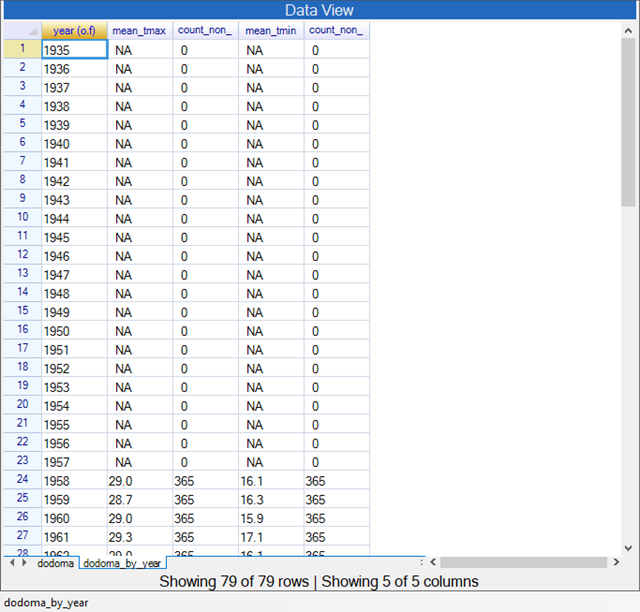 |
Fig. 21 also shows we now have 2 data frames, one at the daily level and the other with the annual summaries. This second data frame is needed for the graphs.
We have one final small preparatory step to do first. This is because the Year column in the Summary data is a factor column. For the graphs we need it to be numeric again. It is often convenient to have both!
-
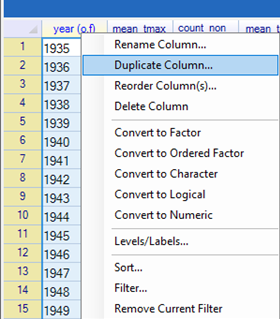
Use Prepare > Data Frame > Duplicate Column... (or right click and choose the appropriate item), Fig. 22.
-
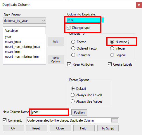
Complete the dialogue as shown in Fig. 23. Press OK to produce another column called year1.
| Fig 22 Right-Click Duplicate Column | Fig 23 Duplicate Dialog |
|---|---|
 |
 |
At last we are ready to produce the graphs.
-
Use Describe > Graphs > Line Plot..., Fig. 24.
-
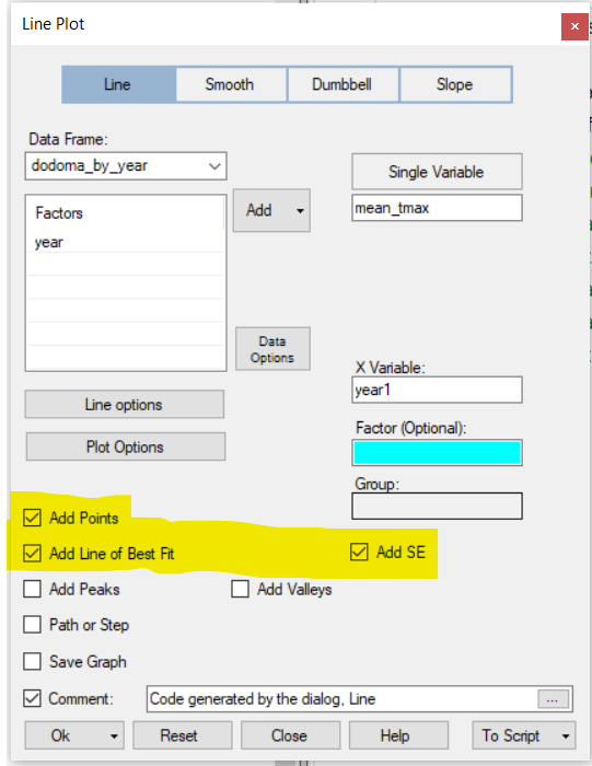
Complete the dialogue as shown in Fig. 25 for the mean_tmin. Press OK.
| Fig. 24 Describe > Graphs > Line Plot | Fig 25. Line Plot dialog |
|---|---|
 |
 |
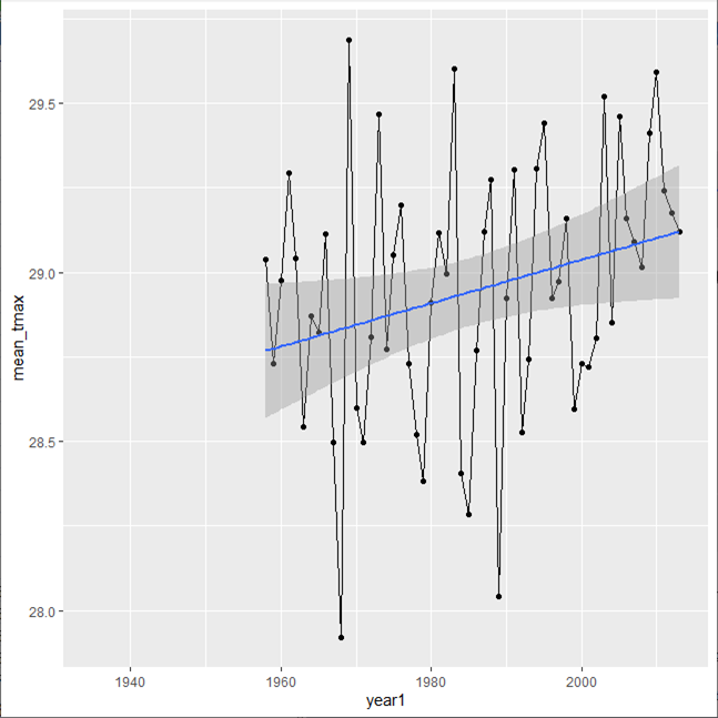
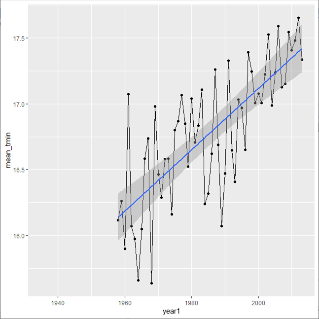
The resulting graph is shown in Fig. 26.
- Return to the Line Plot dialogue and swap mean_tmin for mean_tmax. Press OK to give the second graph also shown in Fig. 27.
| Fig 26 Graph for mean_tmax | Fig 27 Graph for mean_tmin |
|---|---|
 |
 |
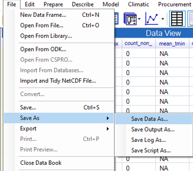
Before using a different data set save these data, so you could resume later.
-
Use the File > Save As dialog, Fig. 28. Choose the option Save Data As.
-
Press on Browse in the dialogue, Fig. 29. Choose a suitable directory and name. Press OK when you return to the Save Data dialogue.
| Fig 28 File > Save As | Fig 29 Saving the Data |
|---|---|
 |
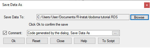 |
The RDS extension is added, to signify it is saved as an R data file. This is the "silver lining" we mentioned in Section 1. If done well, the data only have to be organised once. Then the resulting file, with the two data frames, can be opened in the future, and the analysis can be continued.
There are more analyses that can be explored with this data in R-Instat and we encourage you now to try. The next part of the tutorial focuses on working with labelled data.
R-Instat is still under active development with many improvements and new features planned for future versions. We appreciate feedback you can have to help us improve R-Instat. There are several ways you can provide your feedback:
-
For general feedback you can contact us via email at R-Instat (at) AfricanMathsInitiative.net
-
Our issues page on our GitHub account can be used to report specific bugs or suggestions and this is the most direct way to contact the development team. Note that our issues page is publicly visible to anyone. It can be accessed here: https://github.com/africanmathsinitiative/R-Instat/issues. Click the green New Issue button on the right side to send your message.
When reporting a bug or problem, it's most helpful to us if you can be as specific as possible and detail how to reproduce the bug, pasting the R code from the log file and attaching data if possible.
R-Instat Team, African Data Initiative