Amp Dynamics
The Dynamics plug-in allows you to examine the dynamic performance of a DUT. That is, how the DUT responds to transient events. Newer commercial audio amplifiers are increasingly building in DSP that will compress the incoming signal rather than allow it to distort, and thus the study of these compressors is important. Established standards such as CEA-490 have defined the expected test method for examining a power amp at the limits of its output:
5.2 Dynamic Headroom
The dynamic headroom of a power amplifier (or such section) shall be the ratio of the maximum power output level or a 20 ms burst of a 1 kHz sine wave at the clipping point of the amplifier (see 3.22), to the power output rating (see 5.1), said ratio to be expressed in decibels.
The signal shall be applied at the line input and shall consist of a 1 kHz sinusoidal wave, alternating in level between a nominal level and a level that is 20 dB greater than the nominal level. The signal shall maintain the nominal level for a period of 480 ms ± 10% and shall increase in level for a period of 20 ms ± 10%. The cycle shall repeat with a 0.5 second ± 10% period.
The Dynamics plug-in is focused on looking at peak amplitudes and not distortion. An amplifier that is clipping will fail to display higher peak power, but it can continue to deliver higher RMS power as in the waveform distorts from a sine (RMS = 0.707Vpk) to a square (RMS = Vpk).
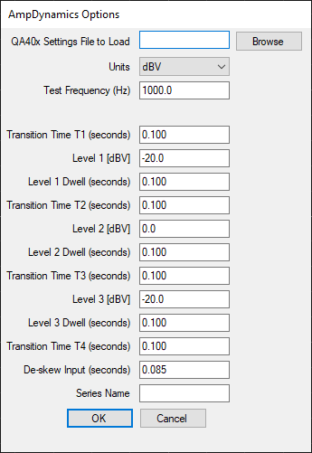
The plug-in is started by going to the Automated Tests menu item and selecting the AMP Dynamics plug-in. The plug-in configuration is shown below.
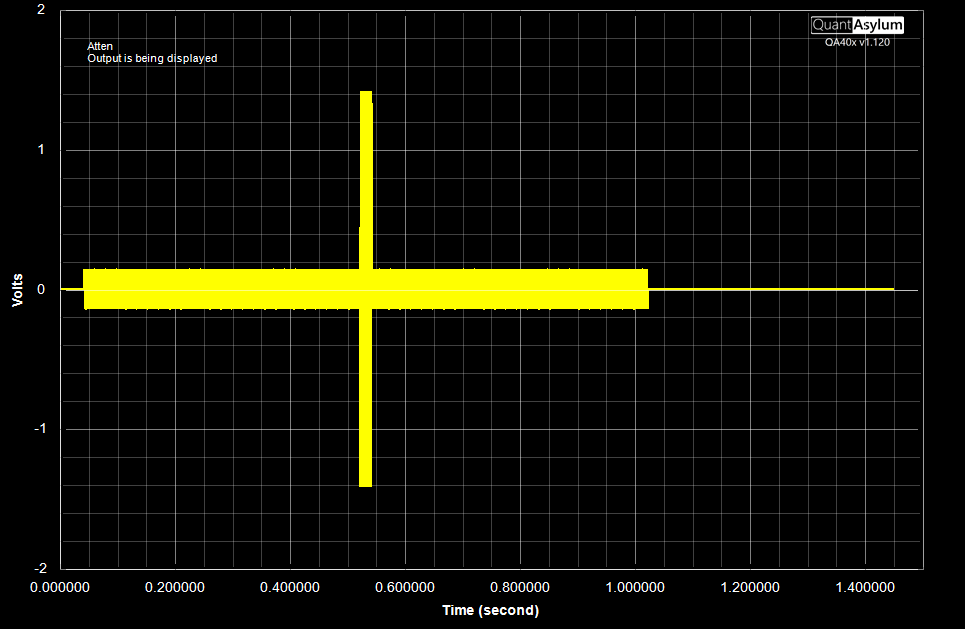
Running the plug-in we can switch to the time domain (Press the Time button in Display Options) and examine the output waveform. That waveform is shown below, annotated with the regions we defined above. The -T indicates a transition region, and the -D indicates a dwell region. Note that the T2-D (Dwell) Level was specified at 0 dBV, and we see the corresponding 1.41Vrms amplitude in the time domain.

The time durations you specify are limited by the maximum FFT size. At 48K, a 1M FFT offers about 21.8 seconds of buffer (1M/48k). If the sum of T1..T4 exceeds that limit, you will receive an error.
In the section above, we looked at the time-domain of the waveform to understand what was being generated. After the plug-in runs, you'll be greeted with a graph that appears as below:

What we see in this graph is the peaks taken inside windows that are twice the period of the stimulus frequency. That is, if you are using a 1 kHz stimulus, then the peak-detection window is 2 mS. So, imagine the time-domain plots divided up into 2 mS segments, and inside each segment you note the peak amplitude.
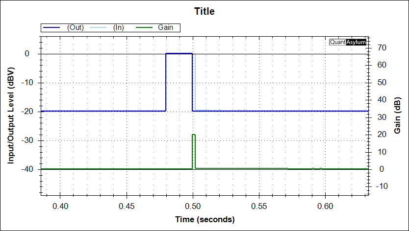
In the plot the output (blue) and input (light blue) are mostly on top of each other, which is expected because the QA402 was in loopback mode. But we can see the 100 mS regions clearly in this plot. We can also see the gain, as determined by comparing the output and the input. Because the QA401 is operating in a linear region, the gain in constant. If you were dealing with an amplifier that was clipping, you'd see the gain as being reduced. We'll show that below as we look at the QA460.
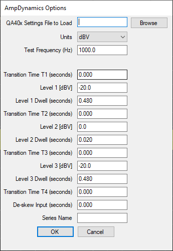
The CEA-490 specification looks at how the dynamic power of an amplifier is specified. Let's set-up a burst so that we have 480 mS of signal at -20 dBV, followed by 20 mS at 0 dBV. We'll use a transition time between the levels at 0 seconds:
The resulting time-domain signals appears as follows:
And the resulting Dynamics plot appears as follows:
Note in the above plot the in and out amplitudes are the same. The input burst appears to linger a bit longer than the input. That is an artifact of the 2 mS window discussed above and can be ignored as the interest here is the amplitude. The artifact also results in an erroneous momentary gain glitch, which can also be ignored.
OK, so let's run that same signal into the QA460 Transducer Amplifier. The maximum output of that amp is around 15 dBV and it has 20 dB of input gain. So the 0 dBV we'll input into that amp would demand a 20 dBV output. But we can see the amp will fall about 5 dB short of that. And the plot of the measurement is shown below:

The plot has had the axis adjusted. But take a look at the gain: We see the gain normally is 20 dB, except for the area we asked the amp to output 20 dBV when we knew the expected maximum was around 15 dBV. In actuality, we can see the amp managed 17.2 dB of output level (that is plateau of the light blue input). But that was short of what was needed, and thus the gain was effectively reduced. This apparent gain reduction is an important part of understanding the health of an amplifier. If RF amplifiers, an amplifier is usually considered "done" when it's operating at its 1 dB compression point. That is, 1 dB below it's expected gain. Beyond that, the amp spectrum is degrading quickly.
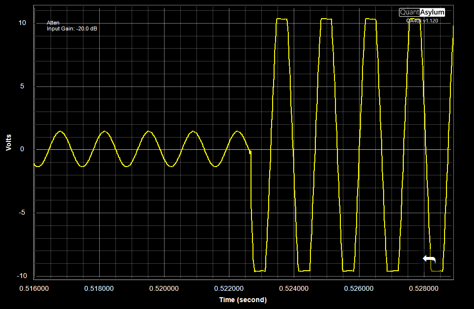
The time domain plot below is a zoom of the transient we injected: The amp responded the only way it knew how, by clipping the tips of the sine:
Compressors are crucial in modern pro-sound audio amplifiers as they help protect the amp during transients that often cannot be anticipated given the realities of live music. But they are also a key part in most all music production. From voice to instrument recording, the chances are great that several compressors were used at various parts of the signal chain.
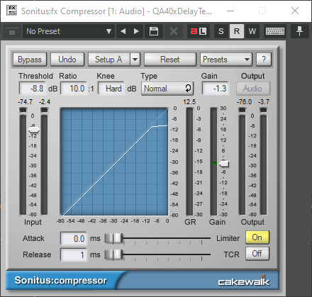
Let's take the stimulus we used above and send that through a compressor with 0 mS attack and decay, and a hard limit. For this test, we'll use a DAW-based compressor.
The waveform looks as follows:

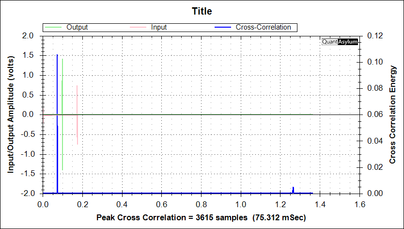
Right away we can see something odd: The output occurs some 100 mS after the input. This is to be expected, because the compressor is an algorithm in the PC, and we're seeing the round trip delay. So, let's run the Path Delay plug-in to learn the precise path delay. Below, we can see it's reported at 75.312 mS.
Now, with that knowledge, let's got back to the Dynamics plug-in and indicate that figure in the de-skew:

And now when we run the Dynamics plug-in again, we see the input and output are better aligned. There's still a bit of a lag which is due to the peak detection envelope. But we can see what the compressor is doing here. That is, once the threshold exceeded the "knee", the compressor pulled back the gain by about 5.5 dB.

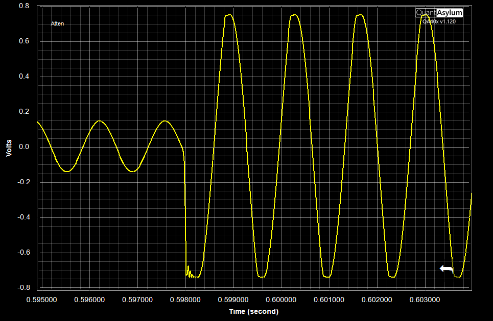
Now, this looks similar to what we saw above in the QA460. But there's a big difference that is apparent when you look at the time domain. And that is that the sine wasn't hard clipped. Instead it was a bit softer:
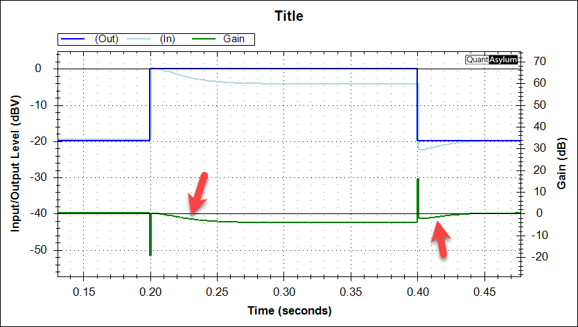
Next, let's look at the compressor in a region it's more commonly used, and that is for controlling longer duration peaks. In plot below, each region has a 200 mS dwell time, and the compressor attack and decay values have been set to 50 mS. The red arrows are indicating the attack and decay response. We can see the gain pull-back started at 200 mS, and was finished by 250 mS. And the release of the gain pullback started at 400 mS, and had been restored 425 mS. So, while the attack pullback looks to be what was requested (50 mS), the release pushback appears to be somewhat shorter.
With the additional peak detection intelligence added and the ability to de-skew the incoming waveform (both added in release 1.13) it should be much easier to see the mechanics of a DAW-based compressor in action.