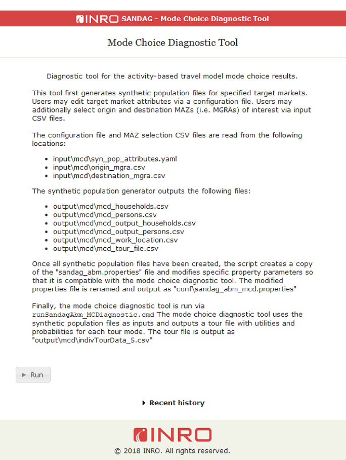
Mode Choice Diagnostic Tool
The mode choice diagnostic tool is intended to help analyze SANDAG's activity-based travel model mode choice results. The tool runs a diagnostic synthetic population covering user-defined origin MAZs (i.e. MGRAs) through the activity-based model in order to visualize tour mode choice probabilities and utilities for a target market population. The synthetic population is generated to cover several user-defined key market segment attributes (e.g. auto ownership, income, educational attainment) and uses default values for other market attributes (e.g. employment statuses, number of persons per household). A file of representative tours (work, shopping) is generated for the synthetic population with pre-determined schedules and destinations. The destination MAZs of interest are user-defined. The activity-based model reads in these generated household, person and tour files and outputs tour mode choice probabilities and utilities for each tour and destination. Finally, a Jupyter Notebook based Python diagnostic visualizer plots, maps and charts results and allows users to query results for sample households, persons, tours and destinations. The following sections describe the setup and application of this tool:
- Process Overview
- Configuring the Mode Choice Diagnostic Tool
- Running the Mode Choice Diagnostic Tool
- Visualizing the Mode Choice Diagnostic Results
The mode choice diagnostic tool is broken up into two main components: a stand-alone mode choice diagnostic Emme tool and a stand-alone diagnostic visualizer.
The stand-alone mode choice diagnostic Emme tool was created using Python and utilizes the pandas and yaml packages to generate the synthetic population. There are 3 main inputs to stand-alone Emme tool: a list of origin MAZs, a list of destination MAZs and a configuration file.
When creating a scenario folder, a mode choice diagnostic (mcd) directory is created within the scenario directory's input directory. The input/mcd directory will contain the 3 input files (listed above), which users can edit. After a successful mode choice diagnostic run, an mcd directory will be created within the scenario directory's output directory. The output/mcd directory will be populated with the output synthetic population files and the final tour mode choice file.
The mode choice diagnostic tool consists of the following procedures:
First, the mode choice diagnostic tool generates a synthetic population using the specified target market attributes from the configuration file along with the list of specified origin and destination MAZs. The resulting synthetic population files are output to the output/mcd directory.
Next, the mode choice diagnostic tool reads the main SANDAG AB Model properties file, modifies a number of property tokens so that it is compatible with the mode choice diagnostic tool, and then saves a copy of the properties file as sandag_abm_mcd.properties. The new properties file is saved in the same directory as the original properties file (conf directory).
Next, the activity-based model reads in the newly generated synthetic population files and outputs tour mode choice probabilities and utilities for each tour and destination. The resulting tour file, along with other mode choice outputs, are output to the output/mcd directory.
Finally, the results of the tool may be queried, visualized, and explored using the SANDAG Mode Choice Diagnostic Visualizer Notebook. Filter the output data by purpose, mode, income, autos, etc. and superimpose the probability and/or utility results over a map of the region.
Configuring the mode choice diagnostic tool involves specifying target market attributes along with desired origin and destination MAZs.
Users may specify attributes for household, person and tour files that will be used to create synthetic population files for target market segments. The target market attributes are set via the input/mcd/syn_pop_attributes.yaml configuration file. Upon scenario creation, the configuration file is populated with default attributes for the mentioned files.
It should be noted that not all synthetic population file attributes may be set. Attributes such as total number of household members or employment statuses are kept as pre-defined fixed values.
Target market households will be generated using the attributes listed in the table below. The total number of household types generated will be determined by every combination of the household income (hinc) and number of vehicles (veh) household attributes. For example, in the configuration file snippet below, there are three values for household income and three values for number of vehicles in household, which totals to nine (3x3) household types. The specified values for the remaining household attributes (household/family type, building size, household unit type) will be applied to all households.
household:

  # household income
  hinc: [14000, 67000, 120000]

  # number of vehicles in household
  veh: [0, 1, 2]

  # household/family type
  hht: 1

  # building size - number of units in structure & quality
  bldgsz: 2

  # household unit type
  unittype: 0
Users must set values for each household attribute where values for household/family type (hht), buidling size (bldgsz) and household unit type (unittype) are limited to their respective attribute categories listed in the table below.
| Attribute | Description |
|---|---|
| hinc | Household income |
| veh | Number of vehicles in household |
| hht |
Household/family type: 0 = Not in universe (vacant or GQ) 1 = Family household: married-couple 2 = Family household: male householder, no wife present 3 = Family household: female householder, no husband present 4 = Nonfamily household: male householder, living alone 5 = Nonfamily household: male householder, not living alone 6 = Nonfamily household: female householder, living alone 7 = Nonfamily household: female householder, not living alone |
| bldgsz |
Building size - Number of Units in Structure & Quality: 1 = Mobile home or trailer 2 = One-family house detached 3 = One-family house attached 4 = 2 Apartments 5 = 3-4 Apartments 6 = 5-9 Apartments 7 = 10-19 Apartments 8 = 20-49 Apartments 9 = 50 or more apartments 10 = Boad, RV, van, etc. |
| unittype | Household unit type: 0 = Non-GQ Household 1 = GQ Household |
Each household has a fixed number of persons (two) where the first person is a worker and the second a non-worker. Therefore, person attributes must contain exactly two values (one for each household member) where the first value corresponds to the worker and the second to the non-worker. For example, in the configuration file snippet below, the first person (worker) is a 35 year-old male who has never served in the military, is not attending school and has a bacehlor's degree. The second person (non-worker) is a 20-year old female who has never served in the military, is a college undergradute and is a high school graduate.
person:

  # age of persons
  age: [55, 20]

  # gender of persons
  sex: [1, 2]

  # military status of persons
  miltary: [4, 4]

  # school grade of persons
  grade: [0, 6]

  # educational attainment of persons
  educ: [13, 9]
Users must set values for each person attribute where values for gender (sex), military status (miltary), school grade (grade) and educational attainment (educ) are limited to their respective attribute categories listed in the table below.
| Attribute | Description |
|---|---|
| age | Age of person |
| sex |
Gender of person 1 = Male 2 = Female |
| miltary |
Military status of person: 0 = N/A Less than 17 Years Old 1 = Yes, Now on Active Duty 2 = Yes, on Active Duty in Past, but Not Now 3 = No, Training for Reserves/National Guard Only 4 = No, Never Served in the Military |
| grade |
School grade of person: 0 = N/A (not attending school) 1 = Nursery school/preschool 2 = Kindergarten 3 = Grade 1 to grade 4 4 = Grade 5 to grade 8 5 = Grade 9 to grade 12 6 = College undergraduate 7 = Graduate or professional school |
| educ |
Educational attainment: 0 = N/A (Under 3 years) 1 = No schooling completed 2 = Nursery school to 4th grade 3 = 5th grade or 6th grade 4 = 7th grade or 8th grade 5 = 9th grade 6 = 10th grade 7 = 11th grade 8 = 12th grade no diploma 9 = High school graduate 10 = Some college but less than 1 year 11 = One or more years of college no degree 12 = Associate degree 13 = Bacehlor's degree 14 = Master's degree 15 = Professional degree 16 = Doctorate degree |
Each person in the household generates exactly one tour. The first person is a worker and generates a work tour. The second person is a non-worker and generates a shop tour. The tour properties specify the start and end period and whether an autonomous vehicle is available for each tour (work and shop). For example, in the configuration file snippet below, the first person (worker) starts and ends their tour at time periods 6 (or between 7:00 and 7:30 A.M.) and 27 (or between 5:30 and 6:00 P.M.), respectively. The second person (non-worker) starts and ends their tour at time periods 19 (or 1:30 to 2:00 P.M.) and 23 (or 3:30 to 4:00 P.M.), respectively. Finally, there is no autonomous vehicle available for the tours.
tour:

  # start period
  start_period: [6, 19]

  # end period
  end_period: [27, 23]

  # av scenario
  av_avail: 0
Users must set values for each tour attribute where values are limited to their respective attribute categories listed in the table below.
| Attribute | Description |
|---|---|
| start_period |
Start Period: 1 = Between 3:00 A.M. and 5:00 A.M. 2 = Between 5:00 A.M. and 5:30 A.M. 3 through 39 corresponds to each half-hour interval between 5:30 A.M. and 12:00 A.M. 40 = Between 12:00 A.M. and 3:00 A.M. |
| end_period |
End Period: 1 = Between 3:00 A.M. and 5:00 A.M. 2 = Between 5:00 A.M. and 5:30 A.M. 3 through 39 corresponds to each half-hour interval between 5:30 A.M. and 12:00 A.M. 40 = Between 12:00 A.M. and 3:00 A.M. |
| av_avail |
Autonomous vehicle availability for the tour: 0 = No 1 = Yes |
In addition to target market synthetic population attributes, users must specify both the desired origin and destination MAZs via the input/mcd/origin_mgra.csv and input/mcd/destination_mgra.csv files respectively. Households will be created for each combination of household income, auto ownership, origin MAZ, and destination MAZ, with two tours (one work and one school) run through mode choice for each household.
The user is cautioned to be selective about the number of MAZs to include in each file, as model runtime and size of the input and output files can quickly exceed resources if too many zones are specified. For testing purposes, we list all microzones in the origin file and 5 selected destinations in the destination file. Model runtime on a SANDAG server was 120 minutes and the output tour file was just under 0.7 GB.
Users may launch the stand-alone mode choice diagnostic Emme tool via the Emme Modeller interface (as described in Run the Model). Within the Emme Modeller, the mode choice diagnostic GUI may be accessed via SANDAG toolbox > Diagnostic > Mode choice diagnostic. To commence the tool, users simply need to click on Run, as is shown in the figure below.
It should be noted that the entire AB model must be run prior to running the Mode Choice Diagnostic Tool so that CT-RAMP inputs (e.g. congested time skims) are available.
Launch the MC Visualizer Jupyter Notebook and configure using the Diagnostic Tool outputs. Users must ensure Jupyter is installed on their system. The mc_utils.py helper file must be in the same directory as the notebook. Users will also need a MGRA shapefile of the study region in addition to the Diagnostic Tool outputs.
Configure the notebook using the outputs from the previous step. Many values can remain unchanged. Note the additional region shapefile requirement that must be sourced separately. Clicking the button will load the input files and check the configuration for accuracy — this can take several minutes depending on the size of the inputs.

Choose from the available options to filter the tool results. The visualizer will plot the utility/probability between the selected zone and all other zones in the tool outputs. The Direction option determines whether the selected zone is an origin zone or a destination zone. The Bins option will automatically default to six equally-sized chunks spanning the range of the utility/probability values. Changing these breakpoints will modify how the results are shaded on the map. The remaining options can further refine the results; selecting All will aggregate (average) all utilities/probabilities across the data dimension.
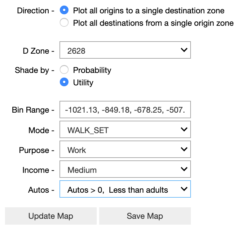
Finally, plot the results with the Show/Update Map button. Depending on the size of the input data and broadness of the filter query, this can take some time to render. If the map does not appear, it may be too large to render inline in the notebook — click Save Map to save the HTML results to your computer. This file can be opened in your browser.
