Predicting Pulsars using the HTRU 2 Data set

To learn about pulsars, watch these two videos-

• https://www.youtube.com/watch?v=gjLk_72V9Bw -This is by NASA's Goddard Space Center
• https://www.youtube.com/watch?v=bKkh7viXjqs - By Astronomate.

I would highly recommend that you read this post:

• https://as595.github.io/classification/

Sample(of size 4) of the data used

#	Mean of the integrated profile	Standard deviation of the integrated profile	Excess kurtosis of the integrated profile	Skewness of the integrated profile	Mean of the DM-SNR curve	Standard deviation of the DM-SNR curve	Excess kurtosis of the DM-SNR curve	Skewness of the DM-SNR curve	target_class
0	140.562500	55.683782	-0.234571	-0.699648	3.199833	19.110426	7.975532	74.242225	0
1	102.507812	58.882430	0.465318	-0.515088	1.677258	14.860146	10.576487	127.393580	0
2	103.015625	39.341649	0.323328	1.051164	3.121237	21.744669	7.735822	63.171909	0
3	136.750000	57.178449	-0.068415	-0.636238	3.642977	20.959280	6.896499	53.593661	0
4	88.726562	40.672225	0.600866	1.123492	1.178930	11.468720	14.269573	252.567306	0

Implementation

In this project, I decided to create a very simple Logistic Regression model (no ResNets be seen) that classifies pulsars.

Ingest and preprocess data

Ingestion

The easiest way to do this would be to add this dataset on Kaggle to your notebook.See how to add data sources here on Kaggle

Otherwise, I have created a tiny script that does it for you, if you are running locally or with other Jupyter notebook providers(ie Google Colab or Binder).

from torchvision.datasets.utils import download_url
import zipfile
data_url="https://archive.ics.uci.edu/ml/machine-learning-databases/00372/HTRU2.zip"
download_url(data_url, ".")
with zipfile.ZipFile("./HTRU2.zip", 'r') as zip_ref:
    zip_ref.extractall(".")
!rm -rf HTRU2.zip Readme.txt

Convert to PyTorch Tensors

1. Create a dataframe(replace PATH_TO_CSV with actual path)

   import pandas as pd
   filename = "PATH_TO_CSV"
   df = pd.read_csv(filename)

2. Convert to numpy arrays- We need to split inputs and outputs.
   Reminder- The output is the target_class

   import numpy as np
   # Inputs
   # This will get everything but the target_class into a dataframe
   inputs_df = df.drop("target_class",axis=1)
   # Convert Inputs
   inputs_arr=inputs_df.to_numpy()
   # Targets-Same thing
   targets_df = df["target_class"]
   targets_arr=targets_df.to_numpy()

3. Convert to PyTorch tensors

   import torch
   inputs=torch.from_numpy(inputs_arr).type(torch.float64)# make sure to not change the types.
   targets=torch.from_numpy(targets_arr).type(torch.long)

4. Create a Tensor Dataset for PyTorch

   from torch.utils.data import TensorDataset
   dataset = TensorDataset(inputs,targets)

Split the dataset

Now we can split the dataset into training and validation(this is a supervised model after all)

1. Set the size of the two datasets

   num_rows=df.shape[0]
   val_percent = .1 # Controls(%) how much of the dataset to use as validation
   val_size = int(num_rows * val_percent)
   train_size = num_rows - val_size

2. Random split

   from torch.utils.data import random_split
   torch.manual_seed(2)#Ensure that we get the same validation each time.
   train_ds, val_ds = random_split(dataset, (train_size, val_size))
   train_ds[5]

3. I would recommend to set the batch size right about now. I am going to pick 200, but adjust this to you needs.

   batch_size=200

   Sidenote- Good time to create data loaders

   I am giving you the option of using a GPU, but I highly do not recommend doing this as you don't need it.

   from torch.utils.data import DataLoader
   # PyTorch data loaders
   train_dl = DataLoader(train_ds, batch_size, shuffle=True, num_workers=3, pin_memory=True)
   val_dl = DataLoader(val_ds, batch_size*2, num_workers=3, pin_memory=True)
   #Transfer to GPU if available
   def get_default_device():
    #Pick GPU if available, else CPU
    if torch.cuda.is_available():
        return torch.device('cuda')
    else:
        return torch.device('cpu')
   def to_device(data, device):
    #Move tensor(s) to chosen device
    if isinstance(data, (list,tuple)):
        return [to_device(x, device) for x in data]
    return data.to(device, non_blocking=True)
   class DeviceDataLoader():
    # Wrap a dataloader to move data to a device
    def __init__(self, dl, device):
        self.dl = dl
        self.device = device
   
    def __iter__(self):
        # Yield a batch of data after moving it to device
        for b in self.dl:
            yield to_device(b, self.device)
   
    def __len__(self):
        #Number of batches
        return len(self.dl)
   device= get_default_device()
   train_dl = DeviceDataLoader(train_dl, device)
   val_dl = DeviceDataLoader(val_dl, device)

Designing the model

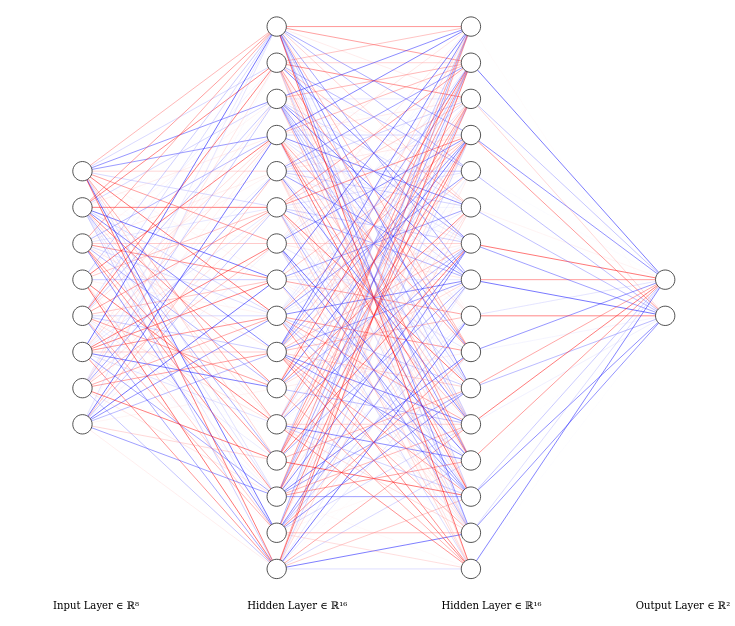
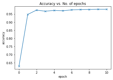
Here I decided to use a simple feed-forward neural network as in testing, it was able to reach a really good validation loss and accuracy.

Specifications of the dataset

• In the dataset, there are 8 inputs and one output
• The output is essentially Boolean value
  • The output is 0 if it is not a pulsar or is 1 if it is a pulsar This would result in 8 neurons for the input layer and crucially two for the output layer. This is because of the Boolean output as mentioned above -one neuron will represent the probability of there being a pulsar and the other will represent the probability of signal interference

Choices:

• Maximum of 16 inner neurons in a layer- performed better than 100 neurons
• Two hidden layers.
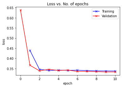
• 10 epochs.
• Adam Optimizer
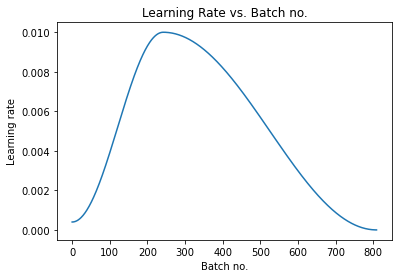
• One cycle policy
• Gradient Clipping(.1)
• Weight decay(1e-4)
• Max learning rate of .1

Create the model class and fit function

Model Class

import torch.nn.functional as F
class HTRU2Model(nn.Module):
    def __init__(self,):
        super(HTRU2Model,self).__init__()
        self.linear1 = nn.Linear(8, 16)
        self.linear2 = nn.Linear(16, 16)
        self.linear3 = nn.Linear(16, 2)
        self.softmax = nn.Softmax(dim=1)
    def forward(self, x):
        x = x.float()# This is necessary or it would cause errors.
        x = self.linear1(x)
        x = F.relu(x)#I prefer to use activations functions like this, feel  
        x = self.linear2(x)
        x = F.relu(x)
        x = self.linear3(x)
        x = self.linear3(x)
        return x
    def training_step(self, batch):
        inputs, targets = batch
        out = self(inputs)                  # Generate predictions
        loss = F.cross_entropy(out, targets) # Calculate loss
        return loss

    def validation_step(self, batch):
        inputs, targets = batch
        out = self(inputs)                    # Generate predictions
        loss = F.cross_entropy(out, targets)   # Calculate loss
        acc = accuracy(out, targets)           # Calculate accuracy
        return {'val_loss': loss.detach(), 'val_acc': acc}

    def validation_epoch_end(self, outputs):
        batch_losses = [x['val_loss'] for x in outputs]
        epoch_loss = torch.stack(batch_losses).mean()   # Combine losses
        batch_accs = [x['val_acc'] for x in outputs]
        epoch_acc = torch.stack(batch_accs).mean()      # Combine accuracies
        return {'val_loss': epoch_loss.item(), 'val_acc': epoch_acc.item()}

    def epoch_end(self, epoch, result):
        print("Epoch [{}], last_lr: {:.5f}, train_loss: {:.4f}, val_loss: {:.4f}, val_acc: {:.4f}".format(
            epoch, result['lrs'][-1], result['train_loss'], result['val_loss'], result['val_acc']))

Fit Function+Other functions

I am applying the one cycle policy. Also I added a little progress bar using tqdm.

from tqdm.notebook import tqdm
def accuracy(outputs, labels):
    _, preds = torch.max(outputs, dim=1)
    return torch.tensor(torch.sum(preds == labels).item() / len(preds))

@torch.no_grad()
def evaluate(model, val_loader):
    model.eval()
    outputs = [model.validation_step(batch) for batch in val_loader]
    return model.validation_epoch_end(outputs)

def get_lr(optimizer):
    for param_group in optimizer.param_groups:
        return param_group['lr']

def fit_one_cycle(epochs, max_lr, model, train_loader, val_loader,
                  weight_decay=0, grad_clip=None, opt_func=optim.Adam):
    torch.cuda.empty_cache()
    history = []

    # Set up cutom optimizer with weight decay
    optimizer = opt_func(model.parameters(), max_lr, weight_decay=weight_decay)
    # Set up one-cycle learning rate scheduler
    sched = torch.optim.lr_scheduler.OneCycleLR(optimizer, max_lr, epochs=epochs,
                                                steps_per_epoch=len(train_loader))

    for epoch in range(epochs):
        # Training Phase
        model.train()
        train_losses = []
        lrs = []
        for batch in tqdm(train_loader):
            loss = model.training_step(batch)
            train_losses.append(loss)
            loss.backward()

            # Gradient clipping
            if grad_clip:
                nn.utils.clip_grad_value_(model.parameters(), grad_clip)

            optimizer.step()
            optimizer.zero_grad()

            # Record & update learning rate
            lrs.append(get_lr(optimizer))
            sched.step()

        # Validation phase
        result = evaluate(model, val_loader)
        result['train_loss'] = torch.stack(train_losses).mean().item()
        result['lrs'] = lrs
        model.epoch_end(epoch, result)
        history.append(result)
    return history

Train the model

Define parameters

epochs = 10
max_lr = 0.01
grad_clip = 0.1
weight_decay = 1e-4
opt_func = torch.optim.Adam

Do initial evaluation

history = [evaluate(model, val_dl)]
history

Train

takes ~6 seconds

%%time
history += fit_one_cycle(epochs, max_lr, model, train_dl, val_dl,
                             grad_clip=grad_clip,
                             weight_decay=weight_decay,
                             opt_func=opt_func)

Graphs

---

Credits and Citations

• alexlenail.me for the Neural network design program.

R. J. Lyon, B. W. Stappers, S. Cooper, J. M. Brooke, J. D. Knowles, Fifty Years of Pulsar Candidate Selection: From simple filters to a new principled real-time classification approach, Monthly Notices of the Royal Astronomical Society 459 (1), 1104-1123, DOI: 10.1093/mnras/stw656

Links

• You can use an "image" data set called HTRU1 to achieve the same results(It also has a greater number of entry points at 60,000).
• An easier way to implement this would be to use SKLearn. This would also allow you to use KNN and SVN(and other classifier models) really easily. Check out this awesome data set on Kaggle