PCA Biplots
The PCA plot can show whether your samples separate into groups, what taxa (or groups of tax) are driving this separation, and what taxa are irrelevant for your analysis. More information about how to interpret PCA plots and how they can be used can be found here.
Metadata is not required to use the Biplot function, however metadata is necessary to use the Colored Biplot function.
There are several ways you can filter your data before a biplot is made. Each input is independent of each other, so you can filter by several different methods. Presence (or absence) of a taxonomy column does not influence the filtering.
-
Minimum count per OTU
This filter removes any rows with a maximum count less than the input. Default is 10 to remove any sparse OTUs. -
Minimum count sum per sample
This filter removes any columns that have a lower total sum of counts than the filter. You can visualize which samples are being removed when applying this filter using the Filtering by counts per sample graph under the Filtering plots tab. Red indicates they were removed from analysis. -
Minimum proportional abundance
This filter calculates frequency for each sample (by column) after filters 1. and 2. are applied, and removes any rows that have no frequencies above the threshold. -
Maximum proportional abundance
This filter calculates frequency for each sample, and removes any rows that have no frequencies below the threshold. -
Minimum count sum per OTU
This filter removes any rows that have a lower sum of counts than the filter. You can visualize which rows are removed with the Filtering by counts per row graph under the Filtering plots tab.
Variance cutoff
This filter calculates the variance for each OTU (row), and removes any rows that have lower variance than the filter. Variance is calculated after all other filters, and after the reads have been transformed by the centre-log ratio.
Adjust scale
This changes the scale of the biplot. When set to zero, it shows the relationship between samples (columns), while being set to 1 shows the relationship between OTUs (rows). Data is not filtered from this operation.
You will need to set graph options before clicking the Colored biplot tab. The dropdown menu allows you to choose which column in your metadata file you would like to colour by. You will be prompted to change the data type button if an error is detected. Numbers are allowed in nonnumeric data type, in case you have categorical numeric data (for example, if 0 and 1 represent no and yes).
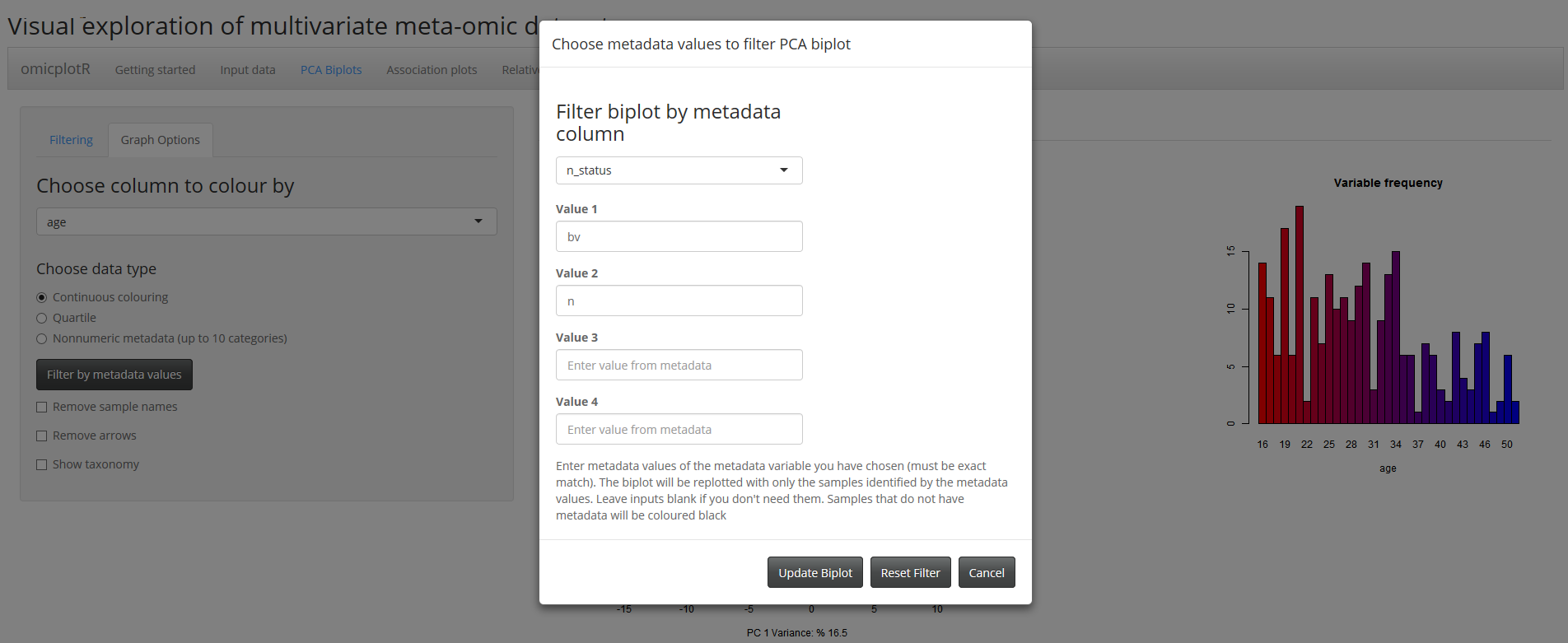
To filter by metadata, click the Filter by metadata values button. In the pop up, you can filter your data based on values from your metadata table. The dropdown menu allows you to choose a column, and you can input the values you wish to recalculate, and plot with a biplot. Any samples not included in these values will be excluded from the calculations and the biplot. Values must be written exactly as in the metadata file. The filter can also be updated or reset. Currently, you can input up to four values. Leave spaces blank if they aren't needed. You can choose to remove the sample names from the biplots (replace with dots), remove the arrows, or show the taxonomy using the checkboxes. If Show taxonomy is selected (and you have a taxonomy column), you can display taxonomic levels as your points. You will be prompted to select the level you wish to display (default is Order).
PCA Biplot and Histogram
Each sample will be coloured the same on each graph. If there is black on the biplot, that means you either have data in without metadata to match, or vice versa. These are not shown in the histogram. NA's in the metadata file will appear black in the histogram.