Home
Granular Rigid Body Simulation Framework: efficient research tools to simulate non-smooth granular rigid body dynamics.
This framework was developed by Gabriel Nützi for studying granular rigid body dynamics in the group of Ch. Glocker at the institute for mechanical systems at the ETH Zurich. This work is based on the thesis:
G. Nützi, Non-smooth Granular Rigid Body Dynamics with Applications to Chute Flows, PhD Thesis, ETH Zurich, Switzerland, 2016, DOI: > 10.3929/ethz-a-010662262


To view this wiki, please use TeX All the Things to render the math properly if you view this on the github wiki page. Use also the TOC extension https://github.com/Mottie/GitHub-userscripts to browse through this wiki.
|
|
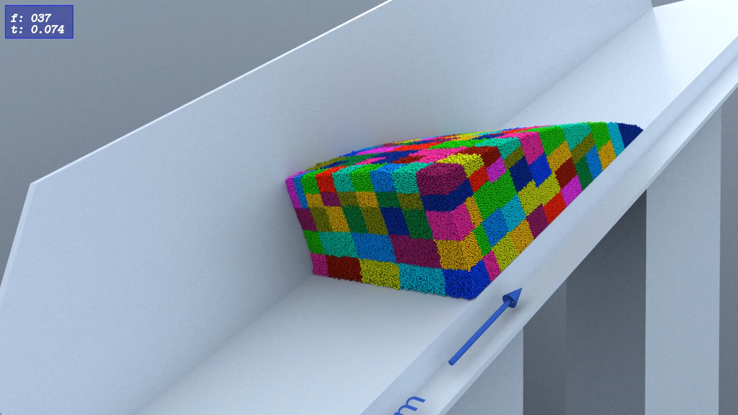 Coloring: Process Domain
|
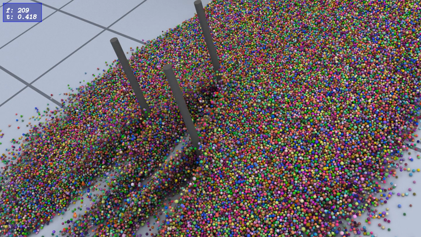 Coloring: Random
|
 Coloring: Velocity
|
Chute flow simulation & experiment with 1 million spheres:
- method: Moreau time-stepping with unilateral contacts and Coulomb friction
- computed on 384 cores with
GRSFSimMPIin 12 h, rendered withGRSFConverterandprmanin 24 h. - time step: 0.0002 s, friction coefficient: 0.8
- restitution coefficient: 0.0 (fully inelastic impacts)
- global contact iterations: 1000
Compiling the rigid body simulators GRSFSim, GRSFSimGUI, GRSFSimMPI and the converter tool GRSFConverter is done by configuring the build with cmake.
To compile the framework, the following dependencies need to be installed as well:
- GRSFSim:
-
GRSFSimGUI (additional to
GRSFSim): -
GRSFSimMPI (additional to
GRSFSim):- OpenMPI: version > 1.5, tested with 1.5 and 1.6, MPI standard 3.0
-
GRSFConverter (additional to
GRSFSim):- HDF5: version > 1.8.15, tested with 1.8.15
- Job Configuration:
Most of the dependencies can either be built from source or directly installed by the system package manager of your operating system. Building from source is recommended due to bug fixes and updates. The framework should compile with gcc-4.9 and with clang-3.6.
Download the repository and configure the build with cmake:
git clone https://github.com/gabyx/GRSFramework.git
git submodule update --init --recursive

mkdir -p build/GRSFramework/release
cd build/GRSFramework/release
cmake ../../../GRSFramework -DGRSF_BUILD_GUI=ON -DGRSF_BUILD_MPI=ON -DGRSF_BUILD_NOGUI=ON -DGRSF_BUILD_SIMCONVERTER=ON
By default the source code of the ApproxMVBB library is assumed to be in the same folder as the folder GRSFramework. The cmake cache variable ApproxMVBB_SEARCH_PATH can be changed or handed to cmake -DApproxMVBB_SEARCH_PATH="../ApproxMVBB" to successfully locate the source code. The source of ApproxMVBB is directly included into the simulators (instead of linked) because it enables better bug fixing.
After cmake has found all dependencies you can build the framework by your IDE or
make -j<N> allwhere <N> is the number of processors to build in parallel. (Take half of your maximum number, since the build uses lots of ram)
You find all executables in build/GRSFramework/release/projects.
The three simulators can be started from the command line right away. Before we go into the details about launching a simulation, the following global environment variable needs to be defined:
export GRSF_REPO_BUILD_DIR="<path-to-your-build-folder>/GRSFramework"Source the following script from the repository root folder:
source <path-to-GRSFramework-repository>/activateThis defines several shortcuts run_sim, run_simgui, run_simmpi and the debugging alternatives run_sim_d, run_simgui_d, run_simmpi_d (if you build the debug versions by configuring the framework in build/GRSFramework/debug)
The interplay between the simulators GRSFSim, GRSFSimMPI, GRSFGUI and the converter GRSFConverter of the framework is best described by the following diagram:

simulations/sceneFileValidation which serves for scene file validation as well as reference. More information about the scene file can be found here SceneFile.
The output of the simulator tools GRSFSim, GRSFSimMPI, GRSFGUI is a binary file .sim containing for each body a generalized displacement \( \mathbf{q} = [{_\mathrm{I}}\mathbf{r}_{S}^\top \ , \ \mathbf{p}_{\mathrm{KI}}^\top]^\top \in \mathbb{R}^7 \) and a generalized velocity \( \mathbf{u} = [{_\mathrm{I}}\dot{\mathbf{r}}_{S}^\top \ , \ {_\mathrm{K}}\boldsymbol{\Omega}^\top]^\top \in \mathbb{R}^6 \).
The vector \( {_\mathrm{I}}\mathbf{r}_{S} \in \mathbb{R}^3 \ \) is the position of the center of gravity \( S \) represented in the inertial coordinate system \( \mathrm{I} \ \) and \( \mathbf{p}_{\mathrm{KI}} \in \mathbb{R}^4 \) is the quaternion describing a rotation from the inertial coordinate system \( \mathrm{I} \) to the body-fixed coordinate system \( \mathrm{K} \).
The term \( {_\mathrm{I}}\dot{\mathbf{r}}_{S} \) is the absolute velocity of the center of gravity \( S \) of the body represented in the inertial coordinate system \( \mathrm{I} \) and \( {_\mathrm{K}}\boldsymbol{\Omega} = {_\mathrm{K}}\boldsymbol{\omega}_{\mathrm{IK}} = \mathbf{A}_{\mathrm{IK}}^\top \dot{\mathbf{A}}_{\mathrm{IK}} \) is the angular velocity of the body represented in body-fixed coordinate system \( \mathrm{K} \).
The matrix \( \mathbf{A}_{\mathrm{IK}} \) is the coordinate transformation matrix from system \( \mathrm{K} \) to \( \mathrm{I} \) and is identical to a rotation \( \mathbf{R}_{\mathrm{KI}} \) which rotates system \( \mathrm{I} \) to \( \mathrm{K} \).
The converter GRSFConverter ( execute run_simconv) is a tool which implements functionalities such as:
-
converting
.simfiles (run_simconv sim -h) -
extracting information from
.simfiles (run_simconv siminfo -h) - produce render output (RIB) of
.simfiles and a scene XML by an execution graph XML which can then be included in a 3d scene to render with a RIB compliant renderer (run_simconv renderer -h) -
analyze
.simfiles with an execution graph XML (run_simconv analyzer -h) -
extract gridded data in HDF5 format from
.simfiles (run_simconv gridder -h)
For a simple demonstration of the framework, the following example goes through the most important aspects. For performing simulations, activate the handy Bash aliases and change the directory to the simulation folder:
cd <path-to-GRSFramework-repository>
source ./activate
GOSIMS
Lets look at the scene file simulations/examples/simple/SceneFileFunnel.xml. Run the graphical visualization GRSFSimGUI by
run_simgui -s examples/simple/SceneFileFunnel.xml -m ../projects/media/ -l ./LocalFolder -g ./GlobalFolderwhich should launch the [graphical user interface](Graphical User Interface):
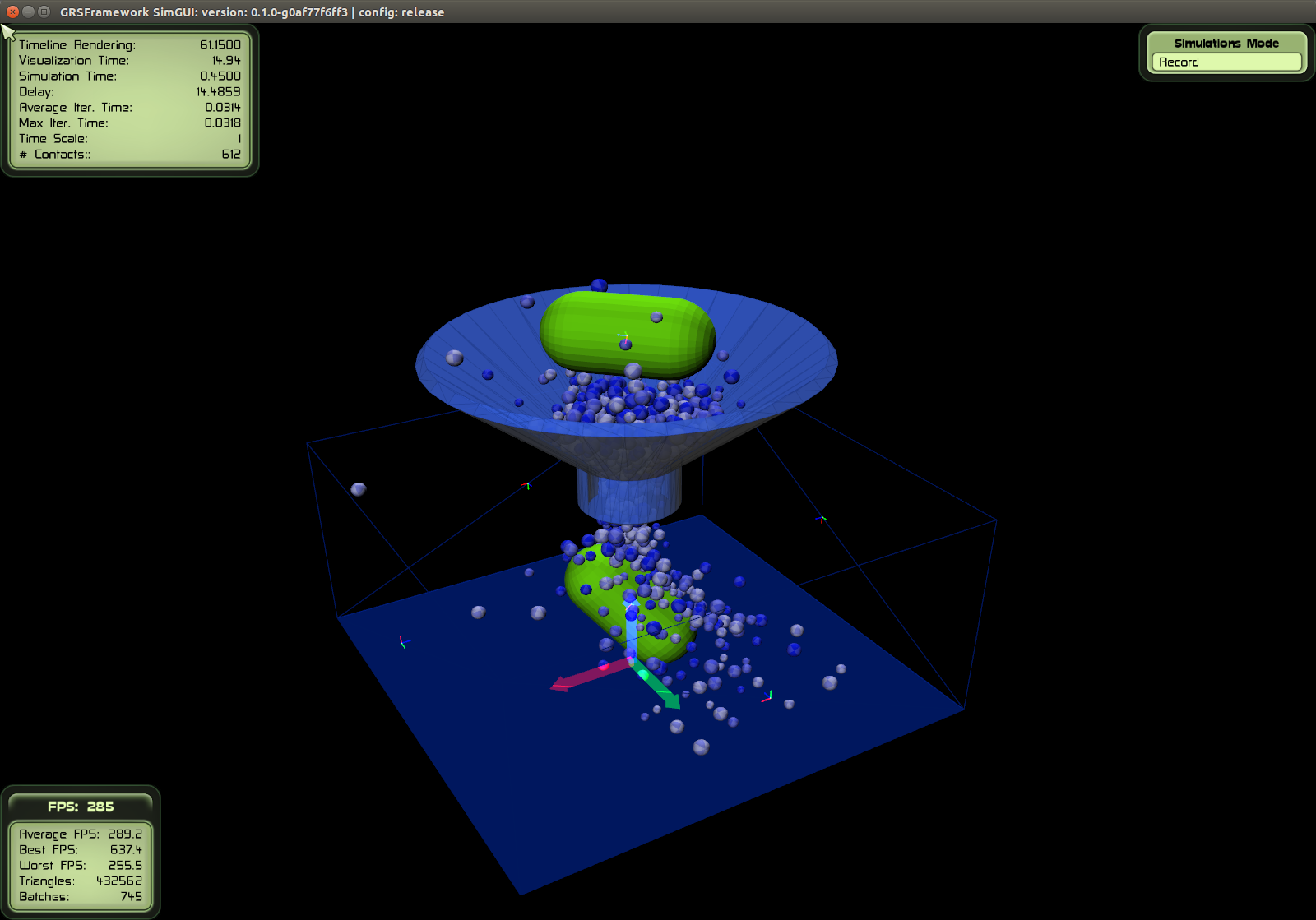
The global folder (option -g) is the output folder for the main output of the simulation, namely the binary simulation file .sim, state data text file .dat, etc. The local folder (option -l) is used for each processes individual files (mainly logs). The local folder is of special use when running the simulation on a high-performance cluster. Meaning that the local folders will resides in the scratch folders of each computing node and the global folder will reference a folder on a parallel file system (i.e. Lustre, Panasas). Since we are launching a single core simulation by run_simgui the local folder will contain only one folder Process_0 after simulating the rigid body system. The graphical user interface is however a two threaded process where one thread is responsible for the graphics and the other is solely responsible for the dynamics simulation.
If you have problems with the graphical user interface, there are three important files for the Ogre graphics engine inside the simulation folder, namely ogre.cfg, plugings.cfg, and resources.cfg. They include some basic settings which should work for all platforms, to reset the settings delete ogre.cfg.
A summarized form of the scene file for the simple simulation is shown below:
<DynamicsSystem
    xmlns:xsi="http://www.w3.org/2001/XMLSchema-instance"
    xmlns="SceneFile"
    xsi:schemaLocation="SceneFile SceneFile.xsd">

<SceneSettings>
    <Visualization/>
    <RecorderSettings mode="everyTimeStep" statesPerSecond="200"/>

    <TimeStepperSettings deltaT ="0.002" endTime="10">
        <InclusionSolverSettings
            method="SORContact"
            ...
            alphaSORProx="1.5"
            ...
            convergenceMethod="InVelocity"
            minIter="1" maxIter="104"
            absTol="1e-6" relTol="1e-6"
            isFiniteCheck = "false"/>
    </TimeStepperSettings>

    <ContactParameterMap>...<ContactParameterMap>
    <GlobalGeometries>
          <Sphere distribute="random" generator="uniform"
                  seed="5" minRadius="0.005" maxRadius="0.01" id="1"
                  instances="10" />
    </GlobalGeometries/>
    <ExternalForces>...</ExternalForces>
    <GlobalInitialCondition>...</GlobalInitialCondition/>
    <MPISettings/>...<MPISettings>
</SceneSettings>

<SceneObjects>

    <RigidBodies name="balls" instances="700" groupId="0"
                 enableSelectiveIds="true" >
        <Geometry>
            <GlobalGeomId distribute="random" id="1" seed="1"
                          startId = "1" endId="10" />
        </Geometry>

        <DynamicProperties>
            <DynamicState type="simulated" />
            <Mass distribute="uniform" value="1" />
            <InertiaTensor type="homogen" />
            <Material distribute="uniform" id="1"/>
            <InitialCondition type="posvel">
                <InitialPosition distribute="grid"
                                 gridSizeX="10" gridSizeY="10" distance="0.03"
                                 translation="0.00 0.00 0.8" jitter="true"
                                 seed="4" delta="0.005"/>

                <InitialVelocity distribute="transrot">
                    <Vel transDir="0 0 -1" absTransVel="1" rotDir="1 0 0"
                         absRotVel="0"/>
                </InitialVelocity>

            </InitialCondition>
        </DynamicProperties>

        <Visualization>
                <Mesh file="Sphere18x18.mesh" scaleLikeGeometry="true"
                      scale="0.0125 0.0125 0.0125" type="permutate" >
                    <Material name="SphereBlue1" />
                    <Material name="SphereBlue2" />
                    <Material name="SphereBlue3" />
                </Mesh>
        </Visualization>

    </RigidBodies>

    <RigidBodies name="floor/ceiling" instances="1" groupId="2">...</RigidBodies>
    <RigidBodies name="sideY" instances="2" groupId="3">...</RigidBodies>
    <RigidBodies name="sideX" instances="2" groupId="4">...</RigidBodies>
    <RigidBodies name="funnel" instances="1" groupId="5">...</RigidBodies>
    <RigidBodies name="capsule" instances="2" groupId="6">...</RigidBodies>
</SceneObjects>
</DynamicsSystem>
The settings and features available in the XML scene file description is best described by an XSD schema. For further information on the scene file description and its validation and the implemented features in the parsers the reader is referred to [Scene File](Scene File).
Scene objects are specified in <RigidBodies> groups which hold a certain amount of rigid body instances.
The specifications in <Geometry> or the dynamic properties (mass, inertia, initial conditions) in <DynamicProperties> mostly have an attribute distribute to specify how the properties are generated for all body instances in this group. For the group with groupId="0" in the above scene file, global geometry ids are randomly generated for their geometry specifications over all 700 bodies (<GlobalGeomId distribute="random" .../>`). The advantage for global geometries is, that they are instanced in each process (for a parallel simulations) and therefore do not need to be communicated among the processes when bodies are changing process domain during simulation.
In the above file, all global geometries are generated by statements inside <GlobalGeometries> such as
<Sphere distribute="random"
        generator="uniform"
        seed="5"
        minRadius="0.005" maxRadius="0.01"
        id="1" instances="10" />
which generates 10 global sphere instances with a uniformly distributed radius between [0.005,0.01] meters with ids in the range [1,11]. Note the global geometry id 0 is not allowed as this value indicates that the body has its own geometry.
The initial position (<InitialPosition>) for the group with groupId="0" specifies a grid initialization which stacks all rigid bodies in this group on a 10 x 10 x ? grid (with some applied position jitter) with grid distance 0.03 where the grid is translated by [0,0,0.8] meters.
The initial condition for the velocities for the group with groupId="0" are specified by specifying translational and rotational velocities (type="transrot") . All <Vel> specifications inside <InitialVelocity> are applied linearly over all body instances in this group and since only one (to few for all 700 bodies) velocity specification <Vel> is given, this single initial condition is applied for all bodies.
After you performed the simulations, start a python notebook by
GOSIMS
jupyter notebook
There is a script to install a complete python virtual environment, see section Python Environment.
You can run the parallel simulation by doing
run_simmpi "-np 4" -s examples/simple/SceneFileFunnel.xml \
            -m ../projects/media/ -l ./LocalFolder -g ./GlobalFolder
which runs the setup on 4 cores by using the Message Passing Interface. You can as well watch the simulation using the playback functionality of the GRSFSimGUI executable.
To configure a parallel job for execution on a high-performance cluster (e.g. ETH Euler/Brutus), the HPCJobConfigurator is used. The HPCJobConfigurator generates a job folder with all necessary files to successfully launch a parallel application. In this case a MPI based rigid body simulation. Configuring a job has the main advantage of organizing and structuring the workflow when parallel computing is performed on a cluster. The configured job folder can be deleted and regenerated. To configure the job folder for this simple example, first clone the repository and activate the HPCJobConfigurator macros, then execute the following
GOSIMS
cd examples/jobs/simple
export MYGLOBALSCRATCH_DIR="$(pwd)/scratch/global"
export MYLOCALSCRATCH_DIR="$(pwd)/scratch/local"
configJob
The configuration script will read Launch.sh and Job.ini and will fail telling us that data/SimState.sim is not found.
The data folder inside $GRSF_SIMULATION_DIR/examples/jobs/simple is the folder where all external resources are either copied or linked to make the job successfully launchable.
Execute the makeAllLinks.sh in the data folder
./data/makeAllLinks.shto link the media folder, copy the additional initial condition SimState.sim and the SceneFileFunnel.xml.
Since a cluster job might use (not in this particular example) lots of different resources from all over the place, it is recommended that the Job.ini file, which describes the job, should only use path strings pointing to the data folder.
Running the alias configJob again, successfully configures two successive jobs in cluster/Launch_SimpleJob.0 and cluster/Launch_SimpleJob.1.
Note that the scene file XML in the second configured job folder cluster/Launch_SimpleJob.1 has been setup such that the simulation continues from the last state of the simulation file output SimState.sim of the first job cluster/Launch_SimpleJob.0. This is achieved by using a special template configurator as specified in the Job.ini file:
[Templates]
...
sceneFile = { "inputFile" : "${RigidBodySim:sceneFileTemplate}",
              "configurator" : {
               "modulePath" : "${General:configuratorModuleDir}/jobGenerators/jobGeneratorMPI/generatorRigidBodySim/adjusterContinue.py" ,
               "moduleName" : "adjusterContinue" ,
               "className" : "AdjusterContinue"
               }
            }
...
which uses the AdjusterContinue class in the adjusterContinue.py script to configure the input file ${RigidBodySim:sceneFileTemplate}.
Launching the MPI jobs with 4 processes as specified in Launch.ini locally on your workstation can be done by executing the launch.sh script
cluster/Launch_SimpleJob.0/launch.shThe output of process.sh launched in parallel inside the launch.sh script goes into $MYLOCALSCRATCH_DIR. When the cluster/Launch_SimpleJob.0/process.sh script finishes, the local scratch folder is copied over to the global scratch folder $MYGLOBALSCRATCH_DIR. This workflow is essentially typical for cluster computing. The local scratch is a local scratch folder on each compute node (consisting of several processors), where the global scratch is mostly a global accessible parallel network storage (Pansas,Lustre, etc.). For the case of a rigid body simulation the global storage should support large files since the output .sim file of s simulation is written to the global scratch (MPI-IO) and quickly becomes greater than 100 Gb.
Killing the job locally can be done by Ctrl+C which sends SIGINT to launch.sh. However, properly terminating should be done by sending SIGUSR2 to the whole process group of launch.sh by doing
kill -USR2 -$(pgrep launch.sh)Note the minus in front of the process id returned by $(pgrep launch.sh).
The above is also what the LSF batch system does when it notifies the job (mostly 10 minutes) before its runtime limit. The command mpirun of OpenMPI so far forwards SIGUSR2, thus the script process.sh ignores additional signals when SIGUSR2/SIGINT is caught. The command mpirun also forwards SIGINT but behaves differently. It waits a bit and then sends SIGKILL which might terminate the cleanup routine if it takes too long. Therefore always terminate by sending SIGUSR2.
in each configured job folder there is a submit.sh and submitAll.sh script which submits the job to the batch system.
The batch system so far configured is Platform LSF which uses the bsub command.
You can adjust this in your Job.ini
Executing a configured job with the HPCJobConfigurator follows the procedure visualized in the following few slides:
<iframe src = "ViewerJS/index.html?page=172#https://rawgit.com/gabyx/HPCJobConfigurator/gh-pages/files/HPCJobConfigurationWorkflow.pdf" width="80%" height="530px" allowfullscreen webkitallowfullscreen></iframe>In this example, we are looking at the simulation study in examples/ for a chute flow consisting of 1 million spheres as shown in the videos.
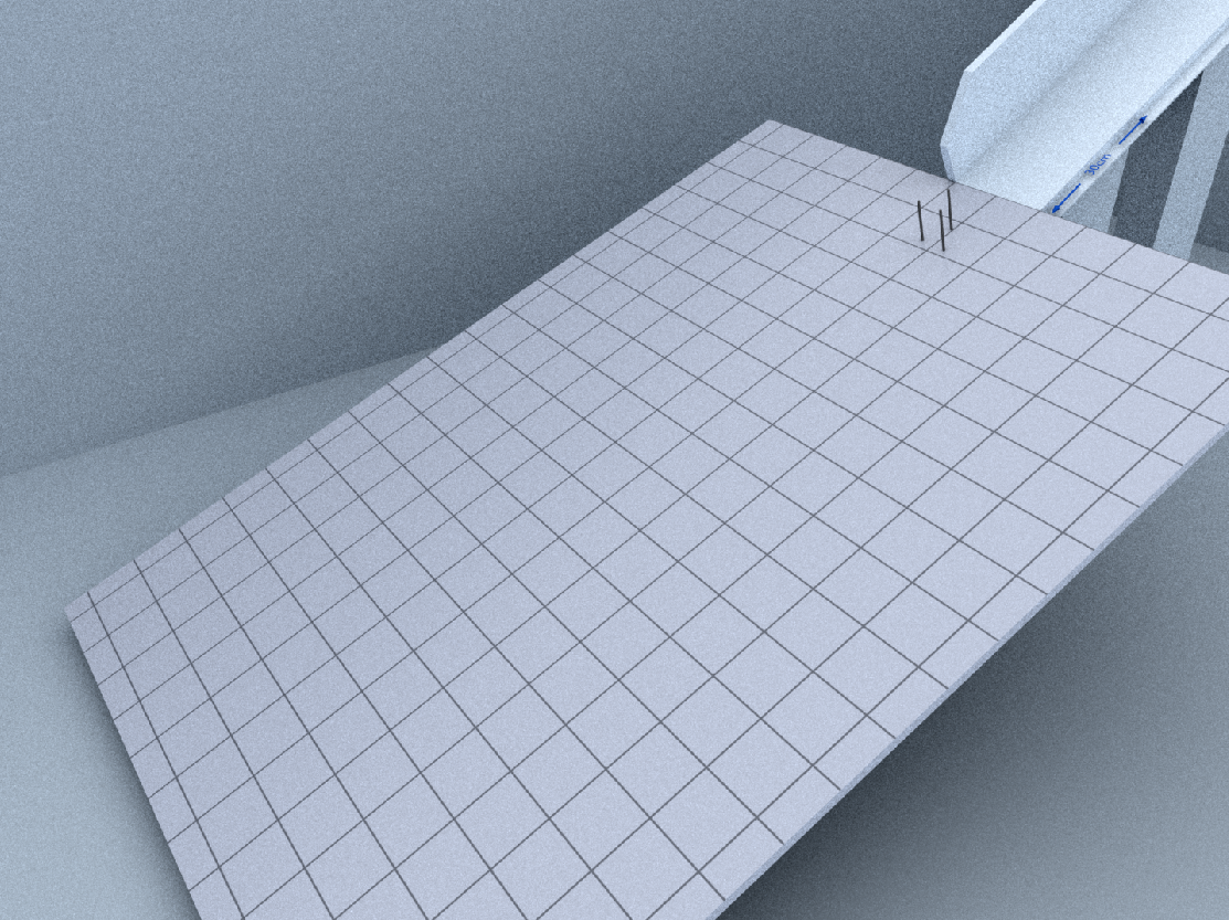
The mechanical model describing this simple simulation is shown below:

This tutorial shows the use of several tools: simulation of a chute flow setup, extraction and analysis of the simulated data and the 3d rendering of the simulation with the render tool of the GRSFSimConverter.
In this example, we look at the parallel jobs (configurable with the HPCJobConfigurator) in the folder
examples/jobs/avalanche1M-Tree-SimStudy in the simulation folder:
cd <path-to-GRSFramework-repository>
source ./activate
GOSIMS
cd examples/jobs/avalanche1M-Tree-SimStudy
To start off, you need to clone the repository which contains the settings and high-speed image data of the experiments:
git clone https://github.com/gabyx/ChuteExperiments.git
export CHUTE_EXPERIMENTS_REPO_DIR="$(pwd)/ChuteExperiments"The parallel rigid body simulations of the chute flow study are located in examples/jobs/avalanche1M-Tree-SimStudy/simulationJobs.
By configuring the simulation jobs with the HPCJobConfigurator as
cd simulationJobs
./config/data/makeAllLinks.sh
python generateAllJobs.py
configures 16 simulation jobs where each job has a slightly different scene file description. In our case, we varied the Coulomb friction coefficient between
the spheres from 0.3 up to 3.
The script generateAllJobs.py script uses the configJob function of the HPCJobConfigurator :
configJob(configFile ="Generator.ini",overwriteArgs=a, colorOutput=True)to build all 16 simulation job folders (each folder ./studies/Avalanche1M-Tree-Study-P-* is a configurable rigid body job analogous to the simple example).
The job folders ./studies/Avalanche1M-Tree-Study-P-{0-15} generated by the generator HPCJobConfigurator.jobGenerators.jobGeneratorSimple.GeneratorSimple specified in Generator.ini are not yet configured. Configuring all 16 simulation jobs (in generateAllJobs.py) is done in the same way by iterating over all simulations jobs ./studies/Avalanche1M-Tree-Study-P-{0-15} and calling
configJob(...), that is
currrentFolder = os.getcwd()
studyFolders = glob2.glob(path.join(currrentFolder,"studies","*"))

for sF in studyFolders:
    os.chdir(path.realpath(sF))
    configJob( overwriteArgs = a, colorOutput=True)
After that, each simulation job ./studies/Avalanche1M-Tree-Study-P-{0-15} can be launched in the same way as the simple example, that is,
  cd studies/Avalanche1M-Tree-Study-P-1
  ./cluster/Launch_Avalanche1M-Trees-Study-P-1.0/launch.sh
which launches the first job of the configured simulation studies/Avalanche1M-Tree-Study-P-1.
In the following, we proceed by only looking at some part of the simulation output of the simulation job studies/Avalanche1M-Tree-Study-P-9.
In the following, we are going to see how to analyze a .sim file with the analyzer tool of the GRSFSimConverter.
We are going to count the number of bodies inside a defined half-space over all simulation states in a .sim file.
This analyzer task is described by an execution node graph (acyclic directed graph).
First define some environment variable to specify the directory which contains some stub .sim file (an extraction of the original simulation P-9)
export AVALANCHE1M_TREES_STUDY_SIMFOLDER="${GRSF_REPO_DIR}/additional/examples/jobs/simulationStudies/simulations/avalanche1M-Tree-SimStudy"To get some information on the .sim file run run_simconv siminfo -i ${SIM_STUDIES_SIM_FILES_DIR}/Avalanche1M-Trees-Study-P-9/SimState.sim.
Now setup the links in the data folder of the analyzer job:
cd examples/jobs/avalanche1M-Tree-SimStudy/analyzerJob
./data/makeAllLinks.sh
Configure the analyzer job by
configJob -x JobAnalyzeStartP-9.ini -p 1The job in cluster/Launch_AnalyzeStart-P-9.0 is generated by HPCJobConfigurator.jobGenerators.jobGeneratorMPI.ToolPipeline specified in Launch.sh. This generator sets up a tool pipeline (templates/PipelineSpecs.json) where each process runs the same tools in the pipeline but with another data set. The embarrassingly parallel work packages are built by scripts/frameGenerator.py. All frames (parallel work packages) are assigned to the number of processes by the job generator. Each frame runs through all tools in the pipeline in a certain process.
A frame in the case of this analyzer job is very simple: it consists of the instruction to analyze one whole .sim file.
Since we have only one .sim file to analyze, this job does not make sense to run in parallel with more than one process (it is an example :-). If you do so, all processes except the first one will immediately return and wait.
Launch the analyzer job as follows :
./cluster/Launch_AnalyzeStart-P-9.0/launch.shwhich will successfully output ${MYGLOBALSCRATCH_DIR}/AnalyzeStart-P-9/AnalyzeStart-P-9.0/Process_0/converter/output/SimState-P-9-FindStart.xml which contains the body count in the lower half-space (after the channel) for all 5 states in the .sim file data/SimState-P-9-0.sim.
The execution node graph can be visualized by the script
${GRSF_SIMULATION_DIR}/python/scripts/GRSFTools/logicExecutionGraphVisualizer/logicVisualizer.py -l analyzerLogic/FindStart.xml -s analyzerLogic/styles.json -o FindStart.svgwhich outputs the following graph:

GRSFSimConverter application) is a little bit overkill for such a simple task as counting the number of bodies in a box. To analyze a rigid body simulation you can of course either design your own execution graph (.xml) and add new nodes of the type LogicNode (see for example the NormNode which computes the norm of a 3-dimensional tuple) to be used in the graph or use the other option: namely write your own custom converter/analyzer code which can be done by looking at the AnalyzerConverter which inherits from SimFileConverter. The converter loop in SimFileConverter accepts visitors (single or multiple ones) whose functions (initSimInfo, initState, addState, addBodyState, finalizeState, isStopFileLoop, isStopStateLoop , isStopBodyLoop get called when stepping over all rigid body states.
So the visitor SimFileExecutionGraph part of the AnalyzerConverter gets handed to its convert function inherited from SimFileConverter.
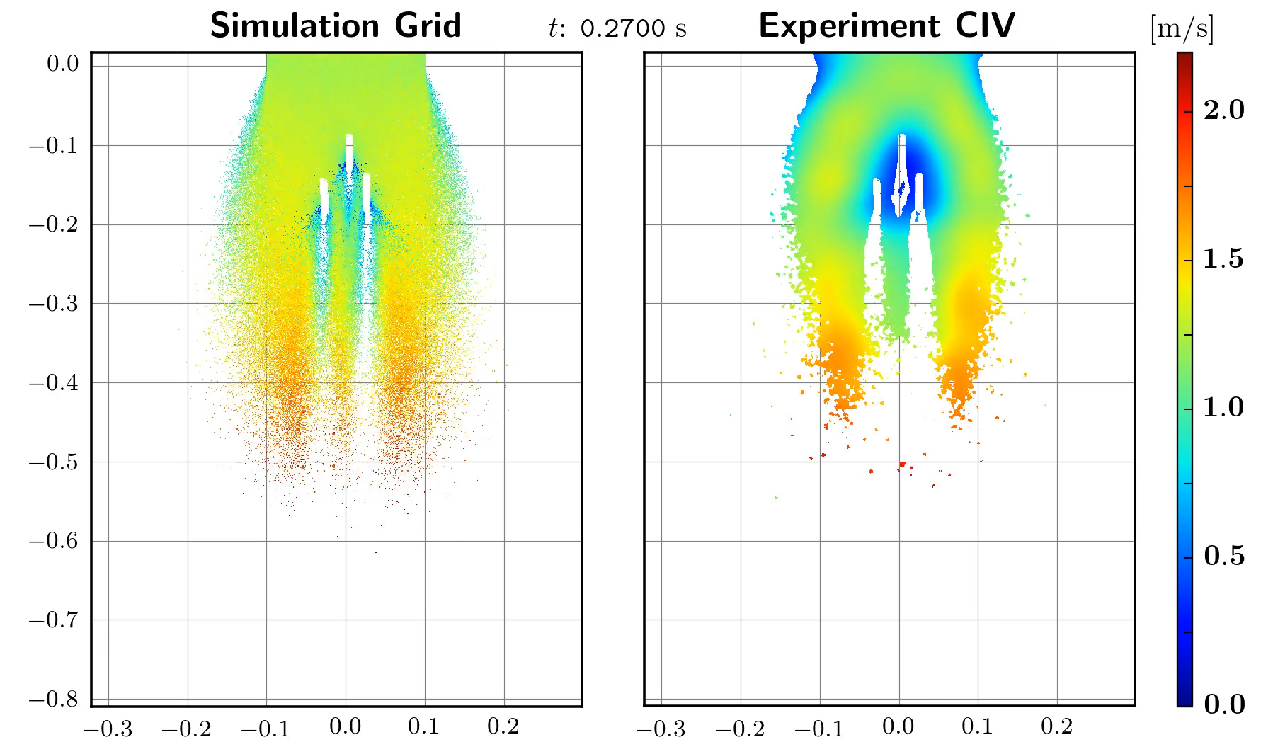
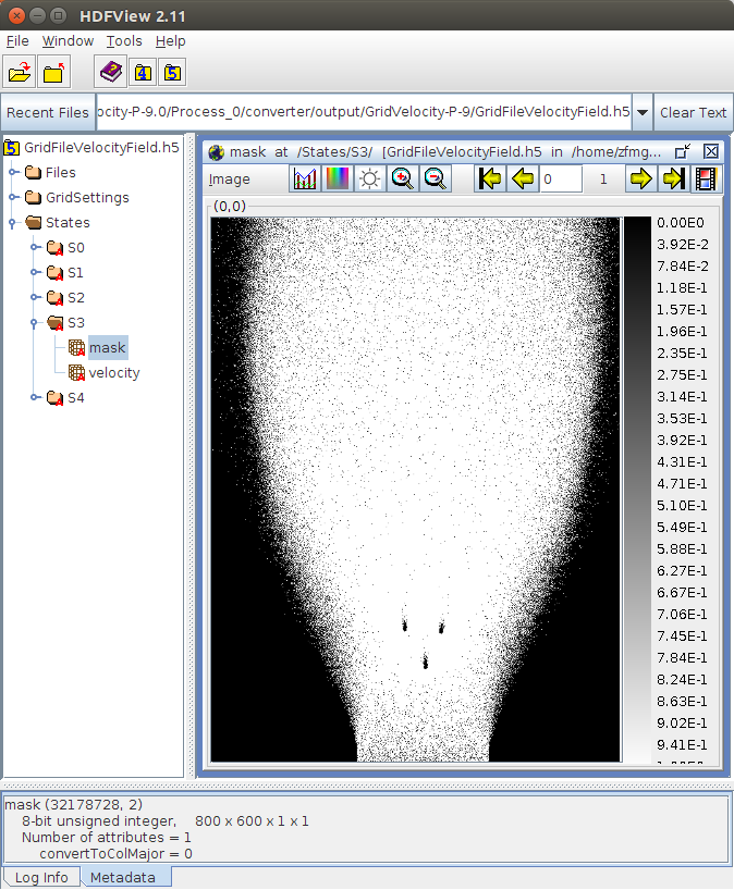
The next job, we are looking at, is the gridder job which uses the gridder functionality of the GRSFSimConverter tool to grid the data of the .sim file output. That means registering certain extractions/computations from the body states into a grid (defined by an OOBB box) in 3-dimensions. The gridder tool also uses the SimFileConverter class for stepping over all states of the .sim file. The logic of the gridder tool is not implemented with an execution node graph but the extraction process is also specified in an XML file. The logic of this specific gridder job is simply to register all rigid bodies in a 800x600x1 grid depending on their center of gravity and taking in each cell only the body with maximum z-component. The extracted grid (.h5 file) contains only the 2-dimensional projection of the velocity vector into the x,y-direction of the grid of the body with maximum z-component (the velocity of the top most body with respect to the z-component of the coordinate system C, see the mechanical model above).
The gridder job is configured by
cd examples/jobs/avalanche1M-Tree-SimStudy/gridVelocityJob
export AVALANCHE1M_TREES_STUDY_SIMFOLDER="${GRSF_REPO_DIR}/additional/examples/jobs/simulationStudies/simulations/avalanche1M-Tree-SimStudy"
data/makeAllLinks.sh # make all links in the data folder
configJob -x JobGridVelocityP-9.ini
The gridder job JobGridVelocityP-9.ini performs the above mentioned data extraction for all states in the data/SimState-P-9-0.sim file starting from the time when the granular material enters the half-space. This is determined by the output of the analyzer job by the linked file data/StudyEntryData.json. Since we do not have all states inside the .sim file of the parameter study P-9 for this demo, the relevant stub file is data/StudyEntryDataP-9Test.json.
The configured job folder contains the string-replaced grid extraction logic XML in cluster/Launch_GridVelocity-P-9.0/GridExtractionLogic.xml:
<?xml version="1.0" encoding="UTF-8" ?>
<Gridder>
  <Logic>
    <GridExtraction fileName="VelocityField.h5">
        <Grid minPoint="-0.80922446 -0.3214161 0"
              maxPoint="0.01756937 0.29867927 1"
              dimension="800 600 1" >
            <Trafo trans="-0.296 0 0"  axis="0 1 0" deg="10"/>
        </Grid>
        <Extract type="TransVelProj2D" name="velocity" indices="0 1" transformToGridCoords="true"/>
        <Extract type="BodyMask" name="mask"/>
    </GridExtraction>
    <!--... more grids of type <GridExtraction> -->
  </Logic>
<Gridder>
The XML above specifies the OOBB specification of the 800x600x1 grid with output file name VelocityField.h5 and two <Extract .../> specifications which produces the above mentioned velocity gridding and a binary mask which contains [0,1] to mark cells which contain at least one body.
Executing the job by
cluster/Launch_GridVelocity-P-9/launch.shresults in a HDF5 file ${MYGLOBALSCRATCH_DIR}/GridVelocity-P-9/GridVelocity-P-9.0/Process_0/converter/output/GridVelocity-P-9/GridFileVelocityField.h5 which can be inspected with the java app hdfview:
Extending the gridder tool of the GRSFSimConverter, can be done by looking at the GridderConverter class which parses and sets up a list of GridExtractor visitors (<GridExtraction> tag in XML) which are then handed to the convert function inherited from also from SimFileConverter.
The GridExtractor contains several extractors (<Extract> tag in XML) inside GridExtractionSettings which can be extended by other fany extractions.
So far the GridExtractor class only registers the body with max z-component. It is to say that the design of the gridder tool is not carefully thought out, but should serve as a starting point for a refactoring.
Rendering a large-scale rigid body simulation is far from easy. If you have your own numerical code for your simulation and just want to use this rendering procedure, you can certainly do so by learning the following demonstrative procedure and using an own specific implementation of SimFileConverter also used for the rendering tool of the GRSFSimConverter. The rendering process has been performed by using Blender 2.76 and the Ribmosaic plugin for the scene modeling and its corresponding RIB export. Renderman Interface Bytestream (RIB) is Pixar's scene description language which has become a standard in the rendering community.
To render the rigid body simulation, the scene is modeled in Blender and exported as RIB files (text files or gzipped text files).
The scene contains certain ReadArchive command hooks which will include RIB description for the granular material we simulated. To provide the RIB description of the granular material, the renderer tool of the GRSFSimConverter is used to generate the output by an execution node graph as for the analyzer and gridder tool.
For our rendering, we used Pixar's free non-commercial Renderman version 20.7.
The render job we will look at in the following can be found in
cd examples/jobs/simulationStudies/avalanche1M-Tree-SimStudy/renderJobYou can either use the Ribmosaic Blender plugin (which is what we used in this demo, produces a RIB compliant export) or the newer PRMan-for-Blender plugin which is the way to go in the future (when using Pixar Renderman) since it includes nodes to design your shaders based on the novel RIS technique. The newer plugin is also able to export RIB files and probably add certain ReadArchive hooks to include the granular material description.
The blender files of the scene for the chute flow simulation can be found in scene/blender/scene.blend. There is a test file scene/blender/sceneRendermanTest.blend which uses the newer plugin. This file is however only for testing RIS shader settings. The Blender file scene/blender/scene.blend was used to produce RIB animations (a RIB file for each video frame). The RIB output can be found in the folder scene/blender/usableRIBSequence for different cameras. All Frame-####·rib in these folders can be straight forward handed to the prman executable and will render a 3d scene of the chute flow simulation without the granular material.
For a small working example, execute
cd examples/jobs/simulationStudies/avalanche1M-Tree-SimStudy/renderJob/scene/blender/usableRIBSequence/scene-staticFar
echo 'Option "searchpath" "string archive" [ "@:.:archives:archives/worlds:archives/lights:archives/objects:archives/objects/geometry:archives/objects/materials:../../materials" ]
Option "searchpath" "string texture" [ "@:../../textures" ]' > SearchPath.rib  # make search path for all files (only for test purposes here)
mkdir output
prman -checkpoint 1m -p archives/Frame-0000.rib
which will render to the following EXR file output/Frame-0000.exr:
 Of course, the granular material is not yet rendered since there is a RIB archive `R12001 {ERROR} File GranularMaterial-f-0.rib cannot be opened by RiReadArchive.` which is not found. This missing archive is produced by the render tool in `GRSFSimConverter`. The scene description (spherical geometry + position + shader) for the granular material sums up to about 100mb per frame.
The render job consists of a tool pipeline where each work item is rendering one frame. Rendering one frame consists of producing the RIB file for the granular material and afterwards rendering the scene with Pixar Renderman.
Configure the job for one process (see this section) by
cd examples/jobs/simulationStudies/avalanche1M-Tree-SimStudy/renderJob/
export AVALANCHE1M_TREES_STUDY_SIMFOLDER="${GRSF_REPO_DIR}/additional/examples/jobs/simulationStudies/simulations/avalanche1M-Tree-SimStudy"
data/makeAllLinks.sh # make all links in the data folder
export PRMAN_NTHREADS=4 # number of threads to use for prman process (use only 1 on cluster)
configJob -x JobRender-P-9-StaticFarTest.ini -p 1
Launch the render job by
cluster/Launch_MyRenderJob-P-9StaticFarTest.0/launch.shThis rendering will render only the frame with index 2 of the data/SimState-P-9-0.sim (see settings in JobRender-P-9-StaticFarTest.ini) and will take some time.
You can look in to the $MYLOCALSCRATCH_DIR while the render job is running and see the output of the converter which produced a file GranularMaterial-f-2.rib.
The scene parser implementation SceneParser.hpp, SceneParserGUI.hpp, SceneParserMPI.hpp throws exceptions if parsing fails.
The parser is structured in modules (SettingsModule, ContactParameterModule, ExternalForceModule,GeometryModule, BodyModule, InitStatesModule, VisualizationModule etc. ). Each module is responsible for a certain section in the XML file and is able to parse all data directly into the data storage (DynamicsSystem.hpp) by handing data pointers to the various modules at construction (DynamicsSystem::createParserModules).
The BodyModule (and its dependent modules: GeometryModule, InitStatesModule etc.) is such that it is able to parse only selective bodies from a range/set of body ids. A body id is a 64bit number [groupId,bodyId] where the first 32 bits describe the bodyId and the last 32 bits the groupId.
The features available in the parser can be best understood by looking at the basic modules implementation in SceneParserModules.hpp
The units in the GRSFramework and the scene file description are with out loss of generality assumed to be SI base units.
To validate and check a scene file, download the Xerces2 Java binary.
You can validate a scene file by executing the following java XSD 1.1 validator:
cd <path-to-GRSFramework-repository>
source ./activate
GOSIMS
java -cp <path-to-xerces2-folder>/xercesSamples.jar  jaxp.SourceValidator -xsd11 -a ./sceneFileValidation/SceneFileGUI.xsd -i examples/simple/SceneFileFunnel.xml
which will output mistakes and errors in the xml file.
The output multi-body simulation file is a binary file. Future work includes the use of a netcdf file structure together with MPI-IO.
So far the binary file is self-written and implemented in MultiBodySimFile.hpp and MultiBodySimFileMPI.hpp.
| Size / Type | Description |
|---|---|
headerSize / char |
Header |
nBodies * bodyStateSize / char |
Data |
| Size / Type | Description |
|---|---|
4 / char |
sim file mark: "MBSF"
|
1 / unsigned int |
sim file version |
1 / unsigned int |
number of simulated bodies |
1 / unsigned int |
degrees of freedom \( n_q \) of the generalized coordinates \( \mathbf{q} \in \mathbb{R}^{n_q} \) |
1 / unsigned int |
degrees of freedom \( n_u \) of the generalized velocities \( \mathbf{u} \in \mathbb{R}^{n_u} \) |
1 / unsigned int |
the type of the additional bytes per body data |
1 / unsigned int |
number of additional bytes per body |
amounts to headerSize = 28 bytes.
| Size / Type | Description |
|---|---|
stateSize / char |
State 0 |
stateSize / char |
State 1 |
| ... | ... |
stateSize / char |
State S-1 |
| Size / Type | Description |
|---|---|
1 / double |
state time |
bodyStateSize / char |
BodyState 0 |
bodyStateSize / char |
BodyState 1 |
| ... | ... |
bodyStateSize / char |
BodyState N-1 |
| Size / Type | Description |
|---|---|
7 / double |
generalized coordinates \( \mathbf{q} \in \mathbb{R}^{n_q} \) |
6 / double |
generalized velocities \( \mathbf{u} \in \mathbb{R}^{n_u} \) |
addBytesSize / char |
AddBytes |
amounts to bodyStateSize = 13 + addBytesSize bytes.
Depending on the type of the additional bytes (see Header), the additional bytes per body may contain the following structure (see )
amounts to addBytesSize = 0 bytes.
| Size / Type | Description |
|---|---|
1 / unsigned int (RankIdType) |
the process rank to which this body belongs |
amounts to addBytesSize = 4 bytes.
| Size / Type | Description |
|---|---|
1 / unsigned int (RankIdType) |
the process rank to which this body belongs |
1 / unsigned int (RigidBodyBase::BodyMaterialType) |
the material id assigned to this body. |
amounts to addBytesSize = 8 bytes.
| Size / Type | Description |
|---|---|
1 / unsigned int (RankIdType) |
the process rank to which this body belongs |
1 / unsigned int (RigidBodyBase::BodyMaterialType) |
the material id assigned to this body. |
1 / double |
the total overlap \( \sum_i -g_i \) of all contact gap distances \( g_i \) on this body. |
amounts to addBytesSize = 16 bytes.
| Size / Type | Description |
|---|---|
1 / unsigned int (RankIdType) |
the process rank to which this body belongs |
1 / double |
the total overlap \( \sum_i -g_i \) of all contact gap distances \( g_i \) on this body. |
amounts to addBytesSize = 12 bytes.
| Size / Type | Description |
|---|---|
1 / unsigned int (RankIdType) |
the process rank to which this body belongs |
1 / unsigned int (RigidBodyBase::BodyMaterialType) |
the material id assigned to this body. |
1 / double |
the total overlap \( \sum_i -\frac{1}{2}g_i \) of all contact gap distances \( g_i \). |
1 / unsigned int (RigidBodyBase::GlobalGeomIdType) |
the global geometry id (>0) of the body if it uses a global geometry. |
amounts to addBytesSize = 20 bytes.
The AddBytes data is only written so far when simulating in parallel with GRSFSimMPI. So far, additional bytes per body are not written nor read by GRSFSim, GRSFSimGUI. The converter GRSFConverter fully reads the additional bytes.
Big/little endianness is not taken care so far. All bytes are written in the endian format defined by the platform on which the simulation runs.
You can get obtain information about a .sim file by running the siminfo tool of the GRSFConverter:
cd <path-to-GRSFramework-repository>
source ./activate
GOSIMS
run_simconv siminfo -i SimState.sim
which will output something like:
<?xml version="1.0"?>
<SimInfo>
  <SimFile path="SimState.sim"
    nBytes="7135156"
    nSimBodies="700"
    nDOFqBody="7"
    nDOFuBody="6"
    nStates="91"
    nBytesPerState="78408"
    nBytesPerBody="112"
    nBytesPerQBody="56"
    nBytesPerUBody="48"
    addBytesBodyType="0"
    nAdditionalBytesPerBody="0"
    readVelocities="true"
    timeList="0 0.002 0.004 0.006">
    <Resample startIdx="0" endIdx="-1" increment="1">
            <Indices>0 1 2 3 4</Indices>
    </Resample>
  </SimFile>
</SimInfo>The graphical user interface an be launched by for example by:
cd <path-to-GRSFramework-repository>
source ./activate
GOSIMS
run_simgui -s examples/simple/SceneFileFunnel.xml -m ../projects/media/
which results in:
<iframe src="https://player.vimeo.com/video/161632565" width="100%" height="436" frameborder="0" webkitallowfullscreen mozallowfullscreen allowfullscreen></iframe>In the simulation & playback state:
| Key | Function |
|---|---|
| F1 or 0 | Switch between playback and simulation state. |
| A, D, S, W | Move camera left,right,forward,backward. |
| Q, E | Move camera up and down. |
| LMB + ⟷ | Move camera around current orbit point. |
| X,Y | Cycle through all possible orbit points (OrbitCamera.hpp) and reorientate the camera towards the orbit point. |
| R | Change rendering style (wireframe/points/normal) |
| 1 | Toggle between mouse cursor & camera movement. |
| 4 | Show MPI domain decomposition (only grid) if specified in scene file. |
| L | Launch simulation thread. |
| K | Stop simulation thread. |
| M,N | Decrease time scale. A time scale of 1.0 results in simulating in real-time if in Realtime simulation mode or in playback state. |
In the playback state:
| Key | Function |
|---|---|
| 3 | Show/Hide GUI overlay. |
In the simulation state:
| Key | Function |
|---|---|
| 2 | Change simulation mode (Record/Realtime). Record simulates as fast as possible, The mode Realtime simulates according to the set time scale in the left upper overlay. |
There are various scripts and notebooks for visualizing tasks and handling the output from the simulators GRSFSim, GRSFSimGUI, GRSFSimMPI, GRSFConverter. The default python environment should be at least version 3.4. You can install a python virtual environment (want clutter up your systems python) by the help of the Bash script installPythonEnv3.4.sh. Execute the script as
yes "yes" | ./installPythonEnv3.sh /opt/python3.4Env 4which will install a python environment with all needed modules inside /opt/python3.4Env. Make sure you have write/read access rights to /opt/python3.4Env other wise use sudo -E (not recommended). You need to install the HDF5 library (see Dependencies) for the h5py module and define the environment variable HDF5_ROOT=/usr/local/HDF_Group/HDF5/1.8.15/ or similar, depending where you installed HDF5.
The amount of output produced during simulation inside the local (per process) and global folders (per simulation) (see example) is controlled by the files LogDefines.hpp for the GRSFSim, GRSFSimGUI, GRSFSimMPI, GRSFSimConverter.
The framework, by default, compiles with all asserts enabled. All simulations in the videos have been performed with these settings. The asserts (since this library is still in a beta state) should be left enabled to allow proper fixing. For experimental purposes and speed, assert macros used in the GRSFramework can be disabled in the files Asserts.hpp inGRSFSim and GRSFSimGUI and GRSFConverter, GRSFSimMPI.
All applications have signal handlers installed which listen to SIGINT and SIGUSR2 and terminate itself on the receive of such a signal. The signal SIGUSR2 has been used for jobs on the Euler/Brutus cluster at ETH Zurich to successfully terminate a simulation when the batch system requests the job to terminate due to the run time limit (mostly 10 minutes prior to SIGKILL).
Signal handling is implemented in ApplicationSignalHandler.hpp.
Appendix Linear Algebra in Mechanics in the thesis is warmly recommended and gives a brief summary for linear algebra related topics used in dynamics such as coordinate transformation, rotations, dual space, inner product, metric etc.
G. Nützi, Non-smooth Granular Rigid Body Dynamics with Applications to Chute Flows, PhD Thesis, ETH Zurich, Switzerland, 2016, DOI: 10.3929/ethz-a-010662262
The framework is licensed under GNU GPL 3.0.