- This fork of Caffe contains code to train Deep Learning models for the task of object detection.
- Major contribution in this fork include implementation of two layers specific to object detection.
- Layer 1 being bbox_data_layer which reads in images as well as their corresponding annotations.
- Layer 2 being squeezedet_loss_layer which implements the core of Object Detection loss function.
Loss function is the implementation of this paper: https://arxiv.org/abs/1612.01051
For more details pertaining to the loss function, refer this blog post
In the directory proto, you can find all the files necessary for running the models.
For details on setting the variables for test phase in proto/SqueezeDet_train_test.prototxt, have a look at the protobuf message for bbox_data_layer.
./caffe test -model <deploy-prototxt> -weights <weights-file>- For
<deploy-prototxt>, use theproto/SqueezeDet_train_test.prototxt - For
<weights-file>, use theproto/SqueezeDet.caffemodel
git clone https://github.com/kvmanohar22/caffe.git
cd caffe
git checkout obj_detect_loss
Build caffe as usual now. Instructions
- Create the annotation file (
<image_name>.txt) for each image in the training dataset - Each annotation should contain information related to the objects present in that image
- Each annotation file should contain the following information for each object in the image:
xmin ymin xmax ymax class-idx- Here,
xmin,yminare the co-ordinates of the top left corner of the rectangle of bounding box - And,
xmax,ymaxare the co-ordinates of the bottom right corner of the rectangle of bounding box class-idxis the class index to which the object within bounding box belongs to. (Indexing starts from0)
- If an image contains more than one object, then the corresponding annotation file looks like:
<xmin_1> <ymin_1> <xmax_1> <ymax_1> <class_idx_1> <xmin_2> <ymin_2> <xmax_2> <ymax_2> <class_idx_2> ...
- Example: If image file is
2011_000090.jpgand contains one object with co-ordinates3445234215and belongs to class0, the corresponding annotation file should be,2011_000090.txtwith contents,34 45 234 215 0
- This is the layer which reads the images and corresponding annotations to train the model
- Important variables to be set: source and root_folder.
- Each line in the
sourcefile should contain 2 values,<path-to-image> <path-to-annotation> - You can either provide absolute path or relative path in the
sourcefile. - If providing relative path, set the variable
root_folderaccordingly - Hierarchy of Dataset
root_folder/ - Images/ - image_0.jpg - image_1.jpg - image_2.jpg - ... - Annotations/ - image_0.txt - image_1.txt - image_2.txt - ... - Example:
layer { name: "data" type: "BboxData" top: "data" top: "bbox" bbox_data_param { source: '/home/user123/source.txt' batch_size: 2 is_color: true shuffle: true } include { phase: TRAIN } } - This layer outputs two blobs,
- blob
datawhich contains image pixel values - blob
bboxwhich contains the bounding box information, used as input blob tolosslayer
- blob
- Assuming that you have either read the paper or the blog, let's proceed
- Let's assume that the
ConvDetlayer name isconv_xx. - Shape of
conv_xx:[N, C, H, W]N: Batch sizeC: Depth of feature mapH: Height of feature map ofConvDet layerW: Width of feature map ofConvDet layer- Example :
layer {
   name: "conv_xx"
   type: "Convolution"
   bottom: "bottom_layer"
   top: "conv_xx"
   convolution_param {
      num_output: <out_kernels>
      kernel_size: 3
      stride: 1
      weight_filler {
        type: "gaussian"
        mean: 0.0
        std: 0.0001
      }
      bias_filler {
        type: "constant"
        value: 0.01
      }
   }
}
- Step 1: Caffe by default orders the data of a blob in the format
[N, C, H, W]. We permute the top blob ofconv_xxlayer to get a new blob of shape:[N, H, W, C]- Example :
layer {
  name: "permute"
  type: "Permute"
  bottom: "conv_xx"
  top: "permute_conv_xx"
  permute_param {
    order: 0 # N
    order: 2 # H
    order: 3 # W
    order: 1 # C
  }
}
- Example :
- Step 2: Slice the top blob of
permutelayer along last axis to produce three blobs- 1st Slice, Name :
slice_0, Shape :[N, H, W, C0] - 2nd Slice, Name :
slice_1, Shape :[N, H, W, C1] - 3rd Slice, Name :
slice_2, Shape :[N, H, W, C2] - With
N,H,Whaving their usual meanings,Kbeing number of anchors per grid,num_classbeing the number of classes. C0=num_class * KC1=KC2=4 * K- Example :
layer {
  name: "slice"
  type: "Slice"
  bottom: "permute_conv_xx"
  top: "slice_0"
  top: "slice_1"
  top: "slice_2"
  slice_param {
    axis: 3
    slice_point: `C0`
    slice_point: `C1`
    slice_point: `C2`
  }
}
- 1st Slice, Name :
- Step 3: Reshape
slice_0from[N, H, W, C0]to[N, X, Y]producing the top blobreshape_slice_0X=K * H * WY=num_class- Example :
layer {
  name: "reshape"
  type: "Reshape"
  bottom: "slice_0"
  top: "reshape_slice_0"
  reshape_param {
    shape {
      dim: 0
      dim: `X`
      dim: `Y`
    }
  }
}
- Step 4: Apply softmax to the output of
reshapelayer- Be careful with the axis along which softmax is applied, it's NOT the default axis.
- Example :
layer {
  name: "softmax"
  type: "Softmax"
  bottom: "reshape_slice_0"
  top: "soft_reshape_slice_0"
  softmax_param {
    axis: 2
  }
}
- Step 5: Apply sigmoid activation to the blob
slice_1ofslicelayer- Example :
layer {
  name: "sigmoid"
  type: "Sigmoid"
  bottom: "slice_1"
  top: "sig_slice_1"
}
- Example :
- This layer takes in 4 blobs as input and produces a single output blob which contains loss.
- The 4 blobs in order are as follows:
soft_reshape_slice_0sig_slice_1slice_2bbox
- Set the parameters for squeezedet_param
- Example (Network trained as part of GSoC) :
layer {
   name: "loss"
   type: "SqueezeDetLoss"
   bottom: "soft_reshape_slice_0"
   bottom: "sig_slice_1"
   bottom: "slice_2"
   bottom: "bbox"
   top: "loss"
   squeezedet_param {
      engine: CAFFE
      classes: 20
      anchors_per_grid: 9
      anchor_shapes: 377
      anchor_shapes: 371
      anchor_shapes: 64
      anchor_shapes: 118
      anchor_shapes: 129
      anchor_shapes: 326
      anchor_shapes: 172
      anchor_shapes: 126
      anchor_shapes: 34
      anchor_shapes: 46
      anchor_shapes: 353
      anchor_shapes: 204
      anchor_shapes: 89
      anchor_shapes: 214
      anchor_shapes: 249
      anchor_shapes: 361
      anchor_shapes: 209
      anchor_shapes: 239
      pos_conf: 75
      neg_conf: 100
      lambda_bbox: 5
      lambda_conf: 1
   }
}
That's it. Start the training by
cd caffe/build/tools
./caffe train \
-solver <solver-file> \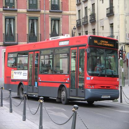
-gpu 0| Original Image | Probability : 84.52% | |
|---|---|---|
 |
 |
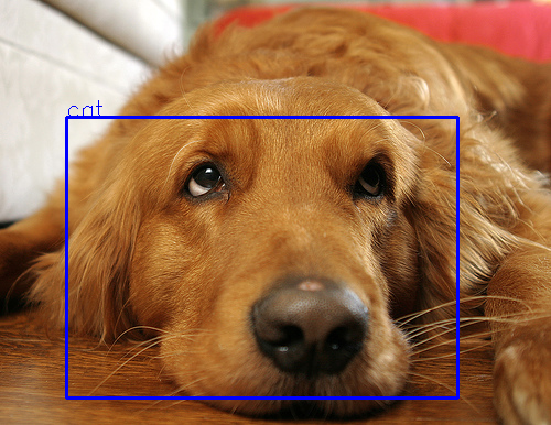
| Original Image | Probability : 70.18% | |
|---|---|---|
 |
 |
| Original Image | Probability : 70.35% | |
|---|---|---|
 |
 |
| Original Image | Probability : 74.51% | |
|---|---|---|
 |
 |
| Original Image | Probability : 73.73% & 72.03% | |
|---|---|---|
 |
 |
| Original Image | Probability : Boat(53.43%) & Person(53.04%) | |
|---|---|---|
 |
 |
I'm exaggerating here. Hmmmm..... I myself couldn't recognize that there was a person out there on the deck !
| Original Image | Probability : Horse(74.26%) & Person(96.26%) | |
|---|---|---|
 |
 |
| Original Image | Probability : 74.12% | |
|---|---|---|
 |
 |
| Original Image | Probability : Train(69.65%) & Person(69.47%) | |
|---|---|---|
 |
 |