Locally Linear Latent Variable Model (LL-LVM) is a probabilistic model for non-linear manifold discovery that describes a joint distribution over observations, their manifold coordinates and locally linear maps conditioned on a set of neighbourhood relationships.
Mijung Park, Wittawat Jitkrittum, Ahmad Qamar,
Zoltan Szabo, Lars Buesing, Maneesh Sahani
"Bayesian Manifold Learning: The Locally Linear Latent Variable Model"
NIPS, 2015
This repository contains a Matlab implementation of LL-LVM. The paper can be found here. A brief summary of LL-LVM can be found in these presentation slides.
Running LL-LVM on a dataset is straightforward. For full demo script see, swissroll_demo.m.
% In Matlab, change directory into the code/ folder.
% Run startup.m to add necessary paths.
%
% Assume that we are given a dataset as a dy x n matrix Y.

% k: k in the k-nearest-neighbours graph construction
k = 9;
% Construct a neighbourhood graph with kNN. n x n matrix.
G = makeKnnG(Y, k);

% options to lllvm_1ep. Include initializations
% Most options are optional. See lllvm_1ep file directly for possible options.
% The only mandatory settings are G and dx.
op = struct();
% The neighbourhood graph as an n x n matrix.
op.G = G;
% The desired reduced dimension. Say we want to reduce to 2 dimensions.
op.dx = 2;

% Call lllvm_1ep to run LL-LVM.
% Relevant output variables are in the struct "results".
[results, op ] = lllvm_1ep(Y, op);

% In particular, results.mean_x is a dx*n x #iterations matrix.
% To get the result x as a dx x n matrix, we can do
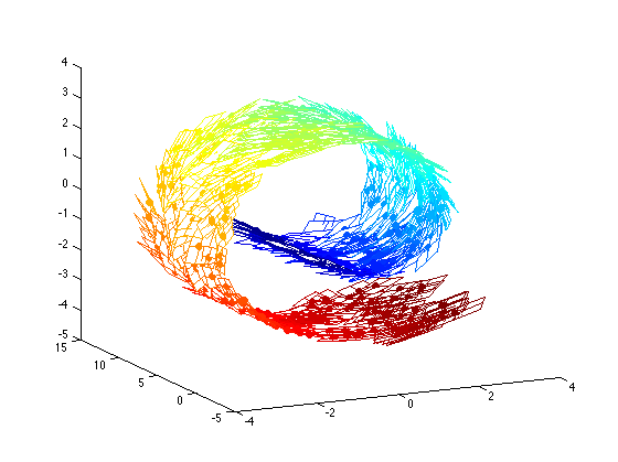
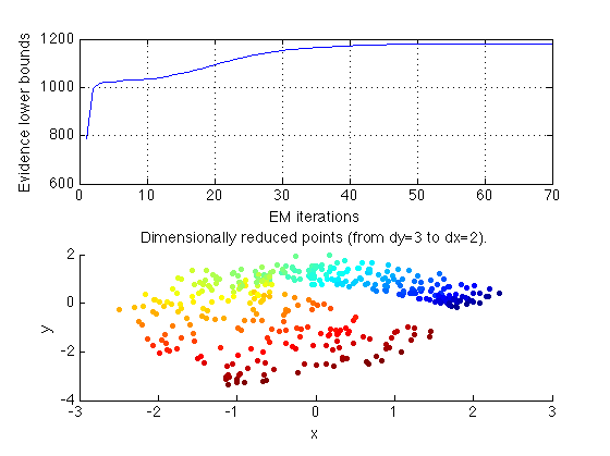
x = reshape(results.mean_x(:, end), 2, []);Assuming that the data Y is a set of points forming a Swiss roll in the three-dimensional space. Here are what we obtain after running LL-LVM. These results can be obtained by running swissroll_demo.m.
Here is the set of local tangent planes learned by LL-LVM.
The following figure shows the evidence lower bounds during the EM, and the dimensionally reduced points in the two-dimensional space.
The unrolling will be cleaner with larger sample size.

