Table of contents

1. Abstract
2. Problem Statement
3. Methodology and Experiments
4. Linear Model
5. Transformer Model
6. LSTM
7. Evaluation and Results
8. Related Work and References
9. Presentation
10. Demo Recording

Abstract

In this project, we are examining article headlines and attempting to quantify how humorous they are. The model uses a continuous scale from 0 to 3 to rank how humorous a particular article headline is. Given an edited and original headline, we aim to predict the average humor score for it using Neural Networks. The process and results of this project can be used for applications such as advancing a machine’s understanding of humor in the English language and could help technologies such as voice assistant jokes.

Problem Statement

The problem involves training a model on thousands of headlines that other people have quantified as humorous or not. In other words, the ground truth is other people’s perceptions of how funny certain headlines are and we use these values to train the model. Our main challenge is to be able to capture the humor in context so that our model can understand why replacing a specific word in a headline makes it funnier.

Methodology and Experiments

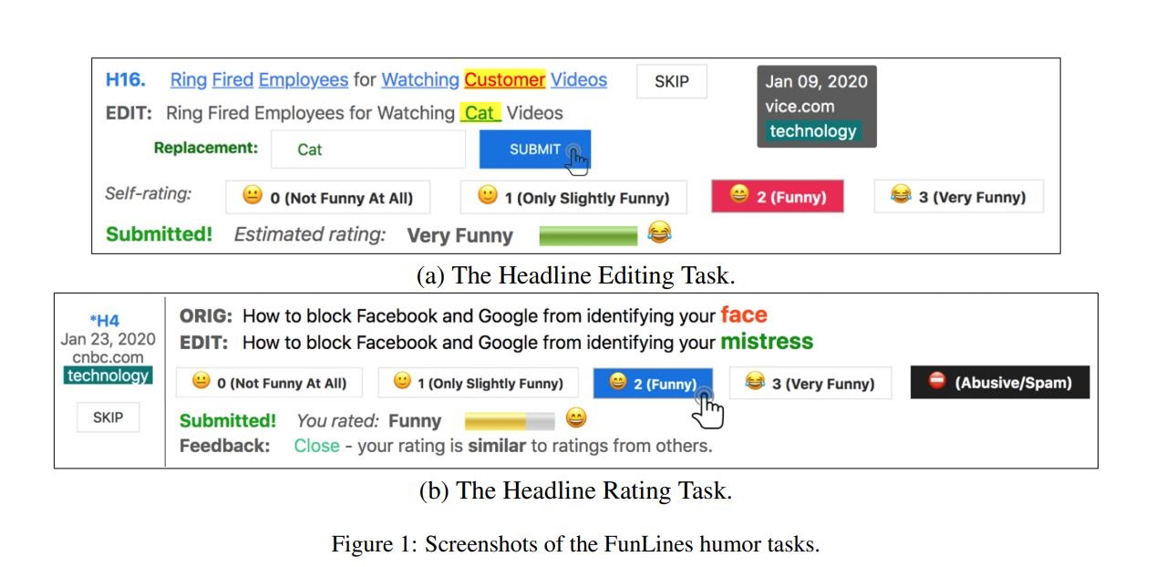
The data we used to train and evaluate our model was curated by the authors of the Rochester paper. They set up a (now defunct) webpage in which they gave study participants a newspaper headline and an edited version of the headline where a single word was replaced with another, and asked participants to evaluate the humor of the transition. An example is the headline "Drilling In America’s ‘Crown Jewel’ Is Indefensible, Former Interior Officials Say," and the replacement of the world Officials with Decorators, which is pretty funny.

Our data consisted of thousands of headlines with a replacement word marked at a certain index within the sentence and 5 humor scores for the word replacement from online survey participants. From this, we were able to separate each entry into the original sentence and the edited sentence, and the mean humor score as our output value.

Linear Model (Fully Connected)

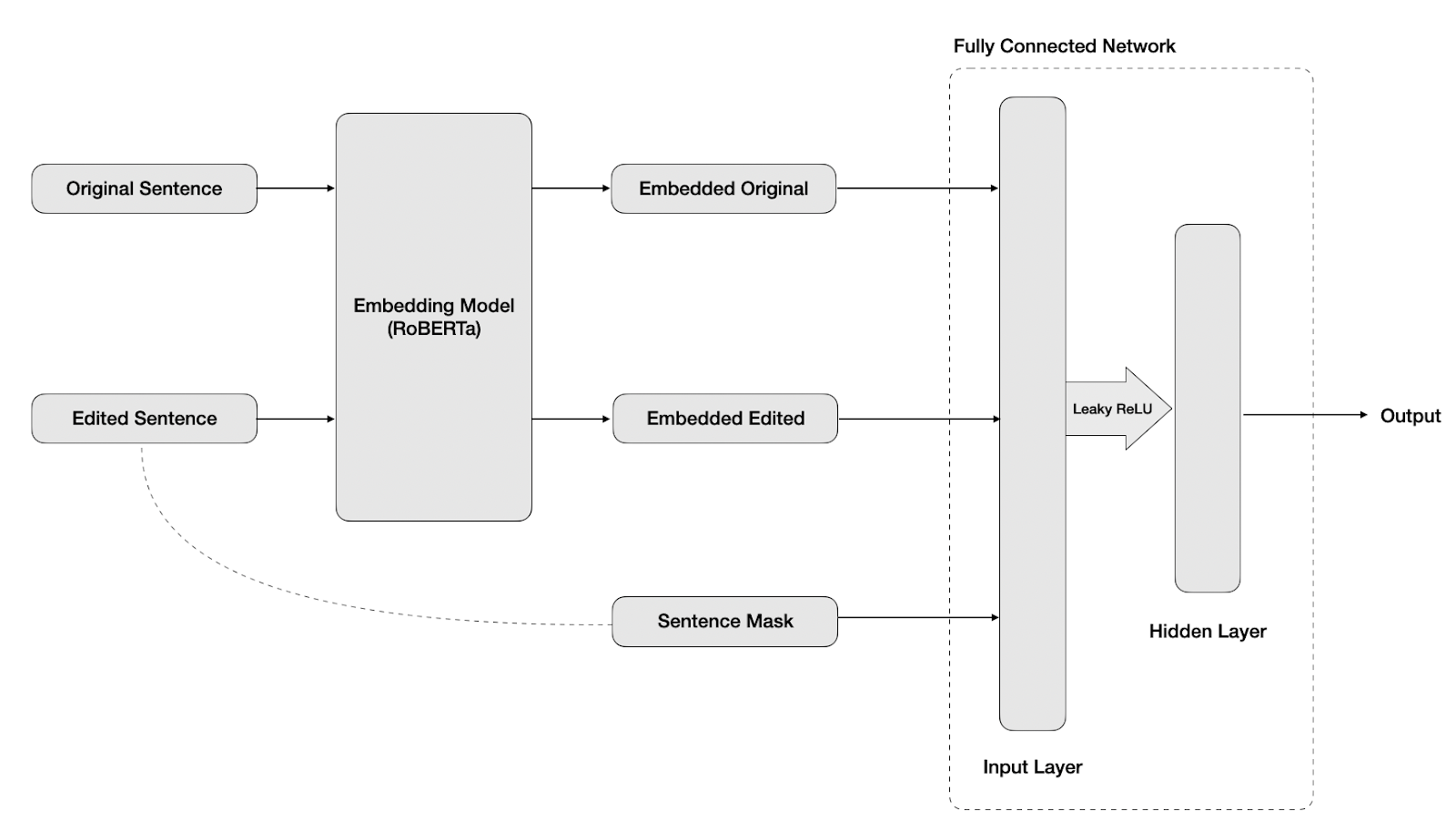
We proposed that we could use an industry standard word embedding model, such as Google’s BERT to calculate contextualized embeddings for each word and use our own deep learning to model the transition from original to edited headline. Initially, we trained a fully connected linear model on the embedded data to predict the mean score. This was a simple model consisting of an input, hidden, and output layer. Our hyperparameters on this model included the size of the hidden layer, batch size, learning rate, and different activation functions.

At first, our model took only the embedding from the edited sentence as an input. However, we realized that much of the humor from edited headlines comes not only from the unexpected edited word, but the transition from the original to the edited headline. In order to represent this transition, we resized our input layer to take a concatenation of {original, edited, masked} headlines, where masked is a vector showing the position of the edited word in the sentence. An example is shown below:

Original: California and President Trump are going to war Edited: California and monkeys are going to war Masked: California and [MASK] are going to war

We also adjusted our hidden layer size to be equal to the dimensionality of the contextualized embeddings and change our activation function from ReLU to leaky ReLU. With this new model architecture, we were able to optimize our hyperparameters and gain a test loss of 0.637, with a train loss of 0.442. This was good, but in order to further improve our model, we proposed that we could gain a deeper level of information using a transformer model on top of multiple embeddings.

Diagram of Fully Connected Model Architecture:

Transformer Model

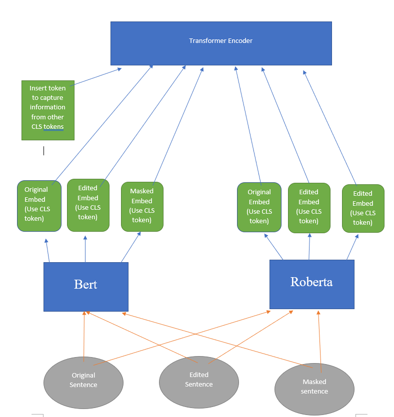
Ensembling multiple pretrained models to do certain tasks in NLP is one of the techniques that people use nowadays. We followed this approach by embedding sentences through Bert and Roberta. To incorporate all the information that we got from Bert and Roberta by using original sentence, edited sentence, and masked sentence, we simply took CLS tokens from embeddings we got from Bert and Roberta, and forwarded them to Transformer Encoder with an arbitrary token in front. We inserted an arbitrary token that went through nn.embedding layer in front of all other tokens before forwarding it to the transformer encoder. Whole idea is that this arbitrary token we inserted will gather information from other 6 CLS tokens that we got from Bert and Roberta by going through a transformer encoder. Since the position of these CLS tokens and arbitrary token does not have any relationship, we got rid of the position encoder.

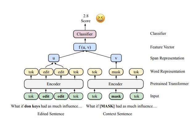
Another approach that we took was using replaced word embeddings instead of CLS tokens from original, edited, and masked sentences. If replaced words were more than one token, we simply averaged those word tokens to get a single word token.

Example of averaging word tokens to get a new word token u

Both of these approaches used two fully connected layers to predict the score using an arbitrary token that we inserted.

LSTM

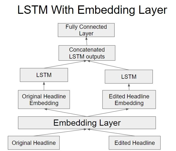
As we explored various options to understand machine humor more, one of our approaches involved trying LSTMs with the original and edited headlines to capture incongruity of the words. Below is our model structure using LSTMs:

Drawing from the original paper as and the transformer experiment in the previous section, we wanted to experiment with training our own embedding layer. We used the original and edited headline as input to the embedding layer and once we had the embeddings we passed each one to its own LSTM to capture the order of the words as it is important to make the headline funny. By concatenating the LSTM outputs and passing it to fully connected layer, we were hoping to capture the relation between the edited and original headlines so we can better predict the humor in the headline

Evaluation and Results

To follow the original findings of the paper, we used MSE loss as our reporting metric. We divided the original dataset into train (80%), dev (10%) and test (10%). Below are the results for the main approaches that we tried.

Model	RMSE (Train)	RMSE (Dev)	RMSE (Test)
Linear	0.442	0.633	0.637
Transformer on CLS token	0.567	0.574	0.563
Transformer on replaced word token	0.565	0.572	0.560
LSTM	0.564	0.568	0.562

Loss for LSTM:

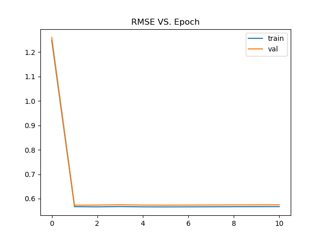
Loss for Transformer on CLS token result:

Loss for Transformer model on replaced word:

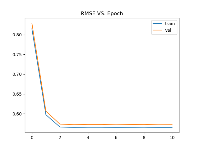
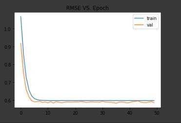
As we can see, Transformer models and LSTM got lowest score on testset compare to devset and trainset. We assume this happened because all of our models are predicting mean score of all scores in trainingset. Thus, it does not matter whether we train or change our network architecture. What it matters is that how far scores are in the dataset. Testset had lowest RMSE score because most of the scores in testset are close to mean score.

Related work and references

The dataset for this project can be found here
In our project we aimed to follow the structure and procedure based on this paper