By Michael Robertson and Aidan O'Neill for Davidson College's Machine Reasoning Homework 1
We implement the A* with three different heuristic functions in an attempt to reproduce the results of Stuart Russell and Peter Norvig in their 2003 paper. We focus on the effect of heuristic choice on the performance of the A* algorithm. Our program generates solvable boards by random moves from the solved position, and reports on the nodes generated by A* as well as the effective branching factor for problems of search depth two to twenty-four. Our results report a smaller average branching factor than Russell and Norvig’s for small problems, but a larger one for larger problems. However, when considering all our data points, we reported correlation values above 0.95, confirming the trends reported by Russell and Norvig. Specifically, we find that that h2 dominates h3, which in turn dominates h1. Lastly, we analyze potential explanations for discrepancies between our results and those of Russell and Norvig.
The 8-puzzle consists of seven tiles and one blank space, and the goal of the game is to arrange the tiles in numerically increasing order, from left to right, top to bottom. A legal move is defined as swapping the tile directly above, to the left of, to the right of, or below the blank square with the blank square.
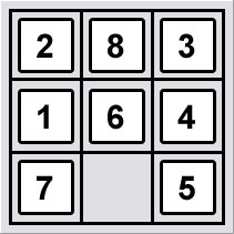
Figure 1: An example of an unsolved eight puzzle
In their work, Russell and Norvig implement the A* search algorithm to solve the puzzle, and report both the memory requirements and effective branching factor for two different heuristic functions (Russell and Norvig 2003). We worked to reproduce their results by writing the A* algorithm in python, and reporting the average number of nodes used by the algorithm, along with the effective branching factor, for problems of even search depth between 2 and 24, inclusive, for three different heuristics generated from relaxed problems. The first of these counted the number of misplaced tiles. The second summed the distances from each piece to its desired position, and the third calculated the number of moves it would take to solve an 8-puzzle in which you can move any tile to the blank square. We define nodes generated as the number of distinct instances of our puzzle class that our heuristic function generates and pushes onto the priority queue used by A*. We define effective branching factor, b*, for a problem with solution depth d and total nodes generated equal to N as
(Russell and Norvig 2003). We will continue to describe our implementation of A*, and then review the ways in which our results support and differ from those of Russel and Norvig. While our broad data trends agree with the results of Russel and Norvig, our exact figures differed slightly, and so we will offer potential explanations for discrepancies.
At first glance, the puzzle seems solvable from any initial state. However, as explained in Johnson’s 1879 paper on the puzzle, all puzzles can be divided into one of two equivalency classes (Johnson and Story 1879). By the even/odd permutation theorem of abstract algebra (Gallian 1986), any permutation must be either even or odd. So, if one forms a permutation by mapping the number of the square to its position on the board, that permutation will either have an even or odd number of cycles, and by Johnson’s analysis, valid moves will change that parity from even/odd to odd/even. Since the sum of the taxicab distances of each piece from its desired solution position also changes its parity with each legal move, we can sum these two numbers whose parity varies with each move to obtain a value whose parity does not vary between boards that are connected by legal moves. Therefore, since this invariant sum is even for the solved board, any board with an even invariant number can be solved, but any odd board cannot.
So, to ensure that the boards we generated were indeed solvable by legal moves, we created an algorithm which produced pseudo-random boards that were always solvable. We began with a solved board state, and then manipulated the board using random legal moves, and ensured that the board never ”back-tracked,” or reentered a state that it had already been in. Because Russell and Norvig’s paper does not describe the process by which they generated random problems of specific depths, we produced our data in a somewhat roundabout way in order to emulate theirs. To solve one hundred problems of depth d, we repeatedly made about 1.3d random moves as described above to produce a pseudo-random solvable board, and then solved it using A*, continuing until we generated one-hundred boards of solution depth d. We will now analyze A*’s efficiency over different heuristics, and compare our results to Russell and Norvig’s. Though our results accurately reproduced their data trends, exact figures differed, and we offer several speculative explanations.
We generated boards by allowing the blank square to randomly walk through the board for a specified number of steps, and then solving the board. For example, to produce boards of solution depth four, we let the blank randomly walk for five moves, and then solved the board using A*, hoping that a high percentage of those boards would have a solution depth of four. After we had recorded the average number of nodes on one-hundred boards of solution depth four, we proceeded to six, then eight, and so forth. For solution depths between 2 and 14, a random walk length of about 1.3d produced results most efficiently, and for depths from 16 to 24, we used a random walk length of 40. We repeated this data gathering process for each of our three heuristics.
We defined h1 as the number of misplaced tiles, not including the blank tile. For example, the unsolved eight puzzle in Figure 1 would have an h1 score of 6, as only the 3-tile and 7-tile are in place. We defined h2 as the sum of the Manhattan distances for the misplaced tiles. For example, tiles in initial positions 1 through 8 for the puzzle in Figure 1 would have an h2 score of
Lastly, we defined h3 from a relaxed 8-puzzle problem, in which a tile can move from square A to square B if B is blank. All three of these heuristics are consistent (Russell and Norvig 2003) and therefore admissible (Ramanujan 2019).
For each data point in figure 2, we increased only counted a node today our sum if we had not previously visited it, or equivalently, placed it in A*’s priority queue. Russell and Norvig’s paper didn’t specify whether they counted a node any time it was generated, or only if it was distinct from all previous nodes and therefore was pushed onto the priority queue, which could account for some differences in our results. In addition, Russell and Norvig did not specify the cost of their path. A*’s priority queue sorts puzzle instances by the value
In our experiment, we set g(n) equal to the path cost, but A* could be modified by weighting g(n) to 1.5 times the path cost, or 3 times the path cost, for example. It is conceivable that Russell and Norvig increased the cost of weighed their path cost more heavily or lightly in comparison to their heuristic, and thereby created fewer nodes than we did. Lastly, Russell and Norvig might have broken ties on the priority queue in a different manner than we did. We broke ties lazily, popping whichever puzzle state was pushed on to the priority queue first in the case that two puzzle states had equal values of f(n). It is possible that Russell and Norvig broke ties differently, say, by popping puzzles with higher g(n) scores off the priority queue first, all else being equal, as puzzles with higher g(n) scores and therefore lower heuristic scores are more likely to be closer to the goal state.
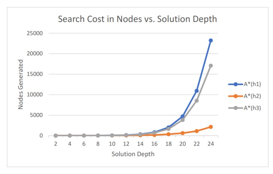
Our results were largely in line with those of Russell and Norvig. The number of nodes we generated to solve the problem had a 99.9% correlation with Russell and Norvig’s forh 1 , and a 98.8% correlation for h2. As we can see from Figure 2, we found that the h2 algorithm consistently outperformed theh 3 algorithm, which in turn consistently outperformed theh 1 algorithm. This difference became increasingly significant as our problem complexity increased in size. From this, we can clearly see how heuristic choice can affect the performance of A*.
Figure 2: The performance of A* when implemented with h1 vs h2 vs h3
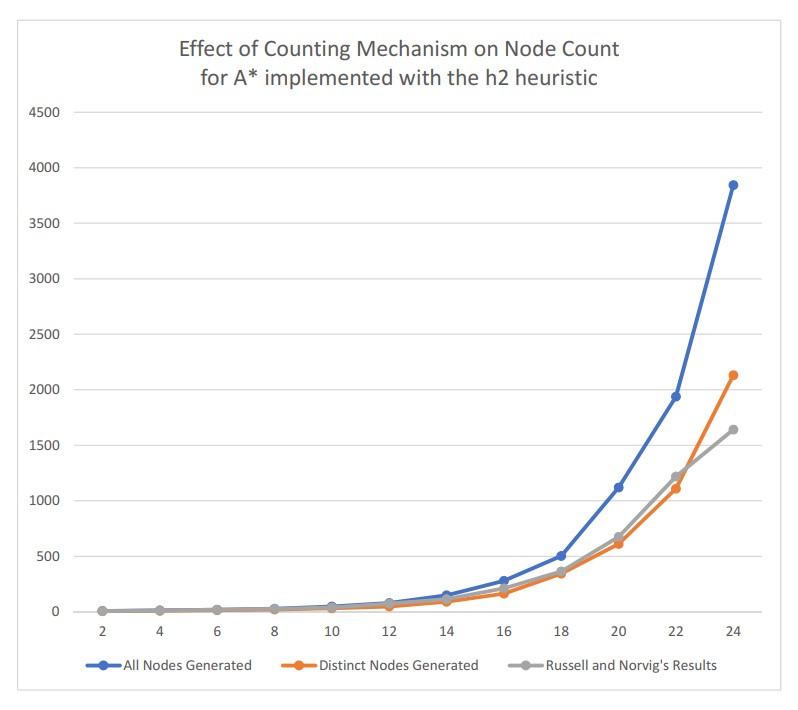
In addition, we can see from Figure 3 how the specific mechanism by which we count nodes affects the results. When we compare our results generated when we count all nodes generated, our results differ greatly from those of Russell and Norvig. However, when we only count distinct board states, our results are much more in line with those of Russell and Norvig, though they differ slightly as the problem size gets more complex around depth 22 and 24.
Figure 3: Change in the number of nodes generated with A* implemented with h2 depending on whether we count distinct nodes or all nodes generated, as compared with the results of Russell and Norvig.
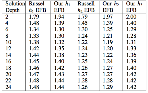
As we see, h2 dominates h3 which dominates h1 : there is no depth of solution for which h1 outperforms h3 and no depth of solution for which h3 outperforms h2. In addition, we must note that our effective branching factor is always slightly different from that of Russell and Norvig. Without access to their code, determining the root of this discrepancy is difficult. It might be how we generated random states - we used "random walks" to randomize the board state for simpler problems with a solution at a lower depth -- moving the blank square in one of the four cardinal directions, and making moves that returned us to a previous state illegal. Of course, there are some board states that would be slightly more likely to occur than others under these rules, but it is possible that we generated slightly harder problems for ourselves than those of Russell and Norvig. In addition, their terminology "nodes generated" is ambiguous in the paper. We counted every successor we generated - Russell and Norvig might have counted their nodes in a different fashion - for instance, when they pushed a node to the heap after checking it against past states. Lastly, they might have weighted their path differently than we did - we used a path weight of one as the cost for any given move, but it is conceivable that Russell and Norvig weighted their path cost more heavily, changing their g(n) function.
Our Effective Branching Factors (EBF) compared to Russell and Norvig's.
Thus, following the work of Russell and Norvig, we wrote an A* algorithm to solve the 8-Puzzle and evaluated the effect of heuristic choice on algorithm performance - clearly, as Russell and Norvig found, the h2 heuristic dominates the h1 heuristic. Further work includes generating truly random states for the problem instead of using random walks for smaller solution depths - perhaps depths generating all possible boards and choosing a board randomly from that set. In addition, we would like to explore more heuristics to see how we can improve on the performance of h2.
We were both equal partners in the process of coding A*. We frequently took turns coding, and we each debugged each other’s work. Michael wrote the Abstract, Introduction, Background and Experiments, and Aidan wrote the Results, Conclusions, Contributions and References section. We both edited the entire paper.
Gallian, J. 1986.Contemporary Abstract Algebra. Pearson Education. Johnson, W. W., and Story, W. E. 1879. Notes on the ”15” Puzzle.American Journal of Mathematics2(4):397–404. Ramanujan, R. 2019. A* with consistency.Davidson College Moodle 2(4):397–404. Russell, S. J., and Norvig, P. 2003. Artificial Intelligence: A Modern Approach. Pearson Education.


