Calculus Basics 微积分基础 #49
Comments
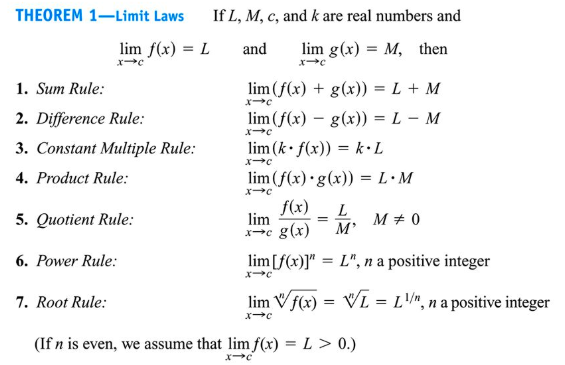
「Limits」 propertiesRefer to Khan academy: Limit properties
The limit of a SUM of functions is the SUM of the INDIVIDUAL limits: Limits of 「Combined Functions」Refer to Khan academy: Limits of combined functions Example
Example
|


Function's Continuity [DRAFT]Pencil Definition: |
Limits
Strategy in finding Limits
|

Limits at 「infinity」No matter why kinds of Limits you're looking for, 「Rational functions」
Refer to previous note on the
Example
Quotients with 「square roots」
Example
Quotients with 「trig」
Example
Easier solution steps:
Example
|


❖ All types of discontinuitiesRefer to Mathwarehouse: What are the types of Discontinuities? 「Jump Discontinuities」
「Removable Discontinuities」
「Infinite Discontinuities」
「Endpoint Discontinuities」
「Mixed Discontinuities」
|


Analyzing functions for discontinuities「algebraic」
At a point Example
|

Application of Removable DiscontinuitiesExample
|

❖ 「Derivative」 Basics
Refer to Mathsisfun: Introduction to Derivatives
A Derivative, is the “Derivatives are the result of performing a differentiation process upon a function or an expression. ” Derivative notationsRefer to Khan academy article: Derivative notation review.
「Lagrange's」 notationIn Lagrange's notation, the derivative of 「Leibniz's」 notationIn this form, we write
How to understand 「dy/dx」This is a review from "the future", which means while studying Calculus, you have to come back constantly to review what the
「Tangent line」 & 「Secant line」
As for the
「Secant line」Example
|


❖ Differentiability
Example of NOT You can see, if the point DOES NOT have 「NOT」 differentiable situations
「Vertical Tangent」We know that the
「Horizontal Tangent」It's a Horizontal Tangent, if:
|


❖ Derivative equationThe idea of derivative equation is quite simple: The LIMIT of the SLOPE.
There're two equations for calculating derivative at a point, and the only different thing is how to express the IMAGINARY POINT with respect to the point
How to calculate 「derivative」Strategy:
Example
Example
|


「Local linearity」 & 「Linear approximation」
Just think of a curve, a good way to approximate its Y-value, is to find another known point near it, and make a line connecting two points, then gets the value by linear equation. Refer to Khan academy lecture.
Example
|


Basic 「Differential Rules」
▼Refer to Math is fun: Derivative Rules
|


Chain Rule
Refer to Khan academy article: Chain rule It tells us how to differentiate
It must be composite functions, and it has to have Common 「mistakes」
How to identify 「Composite functions」
Refer to Khan lecture: Identifying composite functions The core principle to identify it, is trying to re-write the function into a nested one: Examples
Two forms of 「Chain Rule」The general form of Chain Rule is like this: But the Chain Rule has another more commonly used form: Their results are exactly the same. Example
Chain rule for 「exponential function」Formula: Because: Example
|


Derivatives of 「Trig functions」
Reminder of 「Trig identities」 & 「Unit circle」 values# Reciprocal and quotient identities
tan(θ) = sin(θ) / cos(θ)
csc(θ) = 1/sin(θ)
sec(θ) = 1/cos(θ)
cot(θ) = 1/tan(θ)Refer to previous note of all trig identities.
|


❖ Implicit Differentiation
What is 「Implicit」 & 「Explicit Function」Refer to video by Krista King: What is implicit differentiation?
So knowing how to differentiate an How to Differentiate 「Implicit function」Refer to video: Use implicit differentiation to find the second derivative of y (y'') (KristaKingMath) Refer to Symbolab: Implicit Derivative Calculator Assume you are to differentiate
How to differentiate 「Y with respect to X」
How to differentiate 「term MIXED with both X & Y」
Example
Example
Example
Example
「Vertical & Horizontal Tangents」 of 「Implicit Equations」
Example
Example
|


❖ Related RatesJust so you know,
Btw, at Khan academy it's called the Refer to Khan lecture. Strategy:
Example: 「Change of volumes」Refer to previous note of Implicit Differentiation. Solve:
Example: 「Change of volumes」
|


❖ Higher Order Derivatives
「Second derivatives」The second derivative of a function is simply the derivative of the function's derivative. Notation: Second derivatives of 「implicit equations」
Example
Example
|


Derivative of Inverse functions
Derivative of 「Inverse Trig functions」
Example
|


Derivative of 「exponential functions」
Reminder: Don't forget it's a
Derivative of 「log functions」
ExamplesFind the derivative of:
|


❖ Existence Theorems (IVT, EVT, MVT)
Refer to Khan academy: Existence theorems intro
「Intermediate Value Theorem」 (IVT)The IVT is saying:
Refer to Maths if fun: Intermediate Value Theorem Find 「roots」 by using IVT
ExampleTell whether the function
「Extreme Value Theorem」 (EVT)The EVT is saying:
Refer to Khan lecture: Extreme value theorem 「Mean Value Theorem」 (MVT)Refer to Khan academy article: Establishing differentiability for MVT The MVT is saying:
Which also means that, if the conditions are satisfied, then there MUST BE a number
Conditions for applying MVT:
Example
|


❖ L'Hopital's Rule [DRAFT]
From my experience, the L'Hopital's Rule is so often been used that we didn't even realize. Actually it's been used almost every time when we are to evaluate the LIMITS OF RATIONAL EXPRESSIONS.
Example of 「0/0」Example of 「∞/∞」
Example of 「1^∞」L'Hopital Rule for 「Composite functions」Example of composite exponential function
|


❖ Critical pointsRefer to PennCalc Main/Optimization For analyzing a function, it's very efficient to have a look at its
How to find 「critical points」Strategy:
Refer to Symbolab's step-by-step solution. Example
Example
|


❖ Extrema: 「Maxima」 & 「Minima」
And actually we can call them in different ways, e.g.:
How to identify 「Extrema」We need two kind of conditions to identify the Max or Min.
How to find 「Extrema」Refer to Khan academy lecture: Finding critical points We just need to assume 「Increasing」 & 「Decreasing Intervals」We can easily tell at a point of a function, it's at the trending of increasing or decreasing, by just looking at the Finding the 「trending」 at a pointJust been said above, we assume at point Finding a 「decreasing or increasing interval」It's just doing the same thing in the opposite way. Strategy:
Example
How to find 「Relative Extrema」
Refer to khan: Worked example: finding relative extrema
Strategy:
Refer to an awesome article: Using calculus to learn more about the shapes of functions
Example
How to find 「Absolute Extrema」Refer to Khan academy article: Absolute minima & maxima review Strategy:
Example
Example
|


ConcavityRefer to Khan academy: Concavity introduction Two types of concavity: Understand function by 「1st & 2nd Derivative」
Identify 「concavity」 by using 「Second Derivative」
Example
|


❖ Inflection Point
It could be seen as a Algebraically, we identify and express this point by the function's Example
More definitional way to solve:
Example
Example
Example
Example: Finding Inflection points
Example: Finding Inflection points
|


❖ Infinite Seires
Evaluate 「Infinite Series」 as limit of 「partial sums」Evaluate the series, is actually to evaluate the LIMIT of the Example
Example
|


Infinite Geometric SeriesCommon Formula (Finite & Infinite)
Infintite Formula
Determine the Infinite Geometric Series Converges or DivergesThere are two basic rules for infinite geometric series: Example
Evaluate Infinite Geometric SeriesExample
|


❖ Convergence Tests [DRAFT]
「Divergent Test」
「Integral Test」「p-series Test」
「Direct Comparison Test」
「Limit Comparison Test」
「Ratio Test」
「Root Test」
「Alternating Series Test」
「Absolute Convergence」 & 「Conditional Convergence」
|


nth Term Test
Jump over to Khan academy practice: nth term test ▼Here is the divergent test, very simple: Example
|


Integral Test
▼Refer to awesome article from xaktly: Integral Test
「Conditions」 of Integral testAssume the series
「Using」 Integral test
Example
「Understanding」 Integral testThe
As been said above, we got this conclusion:
|


p-series TestFor the the series in form of
▼Refer to xaktly: p-series test/harmonic series 「Harmonic Series」
|


❖ Comparison Test
THIS TEST IS GOOD FOR 「Direct Comparison Test」Assume that we have a series The logic is:
It's so much easier if you think it graphically. ▼Refer to video: Comparison Test (KristaKingMath) ▼Refer to xaktly: Comparison Test Example
「Limit Comparison Test」
The logic is:
► ▼Refer to video: Limit Comparison Test (KristaKingMath) ▼Refer to xaktly: Limit Comparison Test Example
Example
|


Ratio TestTHIS TEST IS GOOD FOR ▼Refer to xaktly: Ratio test / root test
Example
Example
|


Root Test"The root test is used in situations where a series term or part of it is raised to the power of the index variable. "
▼Refer to xaktly: Ratio test / root test
Example
|


❖ Alternating Series TestIt's the test for ►Refer to Khan academy: Alternating series test Alternating SeriesIt means, etc., The Alternating Series Test
The very good example of this test is the
▲ It does CONVERGES. (But the Harmonic Series does NOT converge) Strategy:
Example
Example
|


❖ 「Absolute」 vs. 「Conditional Convergence」
▶Refer to Khan academy: Conditional & absolute convergence
▼We can have a series in We call the series:
etc., Example
Example
Example
Example
|


❖ Error Estimation of Alternating Series
This is to calculating (approximating) an Infinite Alternating Series:
►Refer to The Organic Chemistry Tutor: Alternate Series Estimation Theorem The logic is:
▼Actual sum = Partial sum + Remainder: refer to Khan academy: Alternating series remainder
「Sign」 & 「Size」 of Error►Refer to Khan academy: Alternating series remainder For the
Based on the error's sign,
Bound the Error (accuracy control)The ►Refer to Khan academy: Worked example: alternating series remainder We have 2 ways to bound the error in a range:
Bound by termsThe Larger Strategy:
Bound the errorTo bound the error in a range, we often say:
What they mean are the same: ▲ And by solving the inequality, Example
Example
|


❖ Error Estimation TheoremThe Error Estimation Theorem is not only for alternating series, but available for all infinite series. ▼Boundary of estimating series: refer to Khan academy: Series estimation with integrals
|

❖ Interval of ConvergenceWhen we see the series as a function, we can actually specify an interval for the function so that the series certainly converges over this interval.
The method is kind of like finding the interval of an ordinary function:
Example
|


❖ Power Series
►Refer to Math24: Power series
For easier to remember it, that could be simplified as:
In this function it's critical to know that: Differentiate 「Power series」►Refer to Khan academy: Differentiating power series We have 2 ways to differentiate series, they work same way:
Either way will do, it depends on the actual equation for you to choose which way you're gonna use. Example
Example
Integrate 「Power Series」Example
「Integrals & derivatives」 of functions with 「known power series」
Example
Example
|


❖ Taylor Series
▼Refer to 3Blue1Brown for animation & intuition: Taylor series | Chapter 10, Essence of calculus
►Refer to Khan academy: Taylor & Maclaurin polynomials intro (part 1)
We could expand it and make it clearer ▼: The main purpose of using a etc., we can express the function More importantly, by adding more & more terms into the polynomial, we can approximate the function more precisely: ►Refer to joseferrer: Mathematical explanation - Taylor series
Example
Example
|


❖ Maclaurin Series
▼Expand it we'll understand it better: ▼Here is a graph we're trying to approximate a function centred at Example
Example
Evaluate 「Maclaurin Series」To evaluate a Maclaurin series, we need to convert the series to a function, and then evaluate the function.
|


❖ Lagrange Error Bound
To approximate a function more precisely, we'd like to express the function as a sum of a Taylor Polynomial & a Remainder.
The tricky part of that expression is to "preset" the accuracy of the For bounding the Simply saying, the theorem is:
Example
Example
Example
|


Finding Taylor series for a function [DRAFT]►Refer to Khan academy's unit: Finding Taylor or Maclaurin series for a function |
Function as a 「Geometric Series」Example
|


❖ Maclaurin Series of Common functions►Refer to Wiki: List of Maclaurin series of some common functions Maclaurin series of these common functions are very useful, which we really want to memorize.
Example
Example
Example
Example
|


「Euler's Formula」 & 「Euler's Identity」
▶︎Refer to the most well-known lecture from Sal Khan: Euler's formula & Euler's identity ▼
▼ |


Multivariable functions [DRAFT] |
3D Vector Fileds [DRAFT] |
Parametric Functions [DRAFT] |
Partial derivatives [DRAFT]
|
Gradient [DRAFT]Now we take many
For example: |


Total derivatives [DRAFT]Refer to Coursera: Differentiate with respect to anything
|


Jacobian [DRAFT] |
Directional derivative [DRAFT]
Refer to Khan academy: Directional derivative The So the How to do this:
The
Which comes from:
|


Study resources
Study Tools
Practice To-do List (Linked with Unit tests)
Table of ContentsBasic Differential RulesBasic Integral RulesThe text was updated successfully, but these errors were encountered: