Total Alkalinity measurements at DNR in Olympia

How to conduct Total Alkalinity measurements using the DNR's Mettler-Toledo Titrator in the NRB in Olympia.

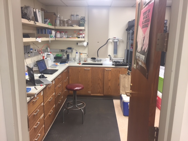
• The lab is located on P1 (Basement level 1) of the Natural Resources Building in Olympia. The key for the lab is located in the aquatics section of DNR, on the 3rd floor, hanging on a hook of cubical 3416, across from Micah's cubical.

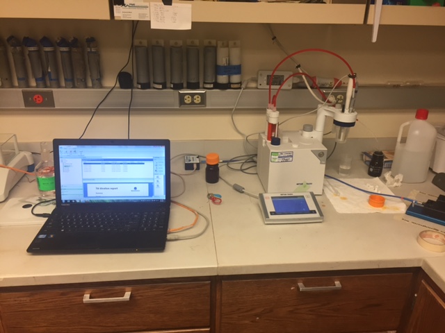
• Begin by turning the laptop on and ensuring the USB cable from the titration is attached to the laptop. Then open the LabX 2014 software located on the desktop. Then turn the titrator on using the switch located on the upper right corner of the machine.

• After the machine has turned on, and located the computer, ensure you have the proper materials.

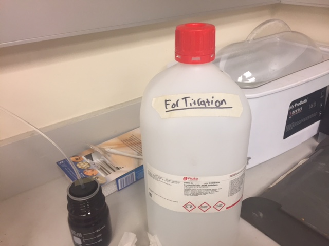
The proper acid to use for titration is 0.1N HCl acid, located in a jug with a red lid, and marked "For Titration". There is a second jug of acid, with a blue lid labeled "For TRIS-buffered seawater" that is 1.0N HCl and produces wildly incorrect results. Be sure to not use this.

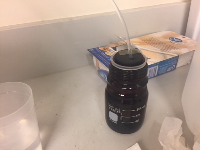
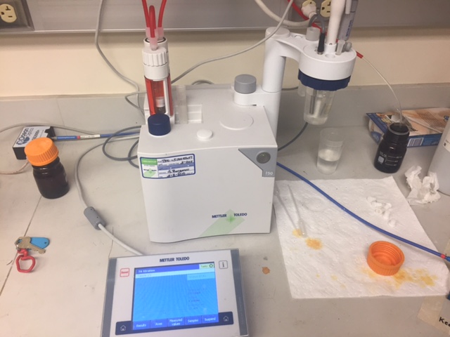
• Fill the small brown jar located behind and to the right of the titrator with acid. This is the titration reservoir. You'll only use ~4 mL per sample, but running out would ruin the sample run, so ensure that it is full.

• After the acid jar is full, grab one of the plastic sample cups located to the left of the sink with "HgCl" written on them and place it in the sample arm. Remove the sample cup with DI water that's attached to the sample arm and place it to the side and wipe the probe and aerator with a kimwipe. Attach the empty cup.

• With the empty cup loaded, go to the titrator screen and run an Acid Purge twice. This purges all of the acid from the pump, drawing new acid in from your fresh acid jar and hopefully purges any bubbles from the line as well. Discard the acid from the cup in the sink to the right.

• Next, recalibrate the probe, to combat day to day drift via:

Steps to recalibrate probe:

1. Obtain 4/7/10 buffer solutions. These are in stock bottles on the left hand side of the upper shelf in the lab.
2. Fill a sample cup ~1/3rd full with each solution. These don't need to be weighed, they just need to cover the pH probe bulb completely.
3. Run the Probe Calibration Method on the Titratior. You'll load the 4.0 buffer, hit ok, then it will run for a while, then load the 7.0 and then the 10.

4. When the calibration has finished it will show a summary screen like:

and the number we're after is the second SLOPECAL value, -58.18mV/pH. This is the number that lets us equate the millivolt readings from the pH probe to the pH of the sample. For reference, last week the SLOPECAL value was -58.90mV/pH so a little change, but not much.

5. After we have our slope value, we need to calculate mV values for pH 3.5, where the initial offgas spin starts, and 3.0, where the titration ends. To do this, we just figure out how many pH units we move from 7 (7 has a mV reading of 0) to 3.5, or 3.5 units, and multiply that time the SLOPECAL value, and get 203.63. Then we calculate our end mV reading, a change of 4 units and get 232.72.

6. These numbers we take to the laptop, and go in to the Analysis Tab, then double click on the New TA Titration method. This brings up a graphical flow chart of the entire process, and we want the "Titration (EQP) [1] method. There we want to check the Predispense Potential, and the Termination Potential values. According to Micah we choose the nearest 10s value to our targets, due to granularity in the dispensing protocol, we won't actually hit exactly 203 or 232. I chose 200, and 230.

• After Calibration , weigh out 60-80 grams of the Certified Reference Material (CRM) sample on the balance into another HgCl marked sample cup. Record this weight, we will need it in the next step.

Note: 60-80g of sample is an important range. If the sample cup is filled too full and the acid input line is submerged, it completes an electrical circuit back to the acid pump, increasing the charge measured by the pH probe, which incorrectly interprets that as a lower pH than intended.

Alkalinity parameters are known to a high degree of certainty for the CRMs, so it's used to ensure the machine is operating properly. Parameters for the individual batches can be found at: http://cdiac.ornl.gov/oceans/Dickson_CRM/batches.html. We'll need to know Salinity later, for the TA calculation in R.

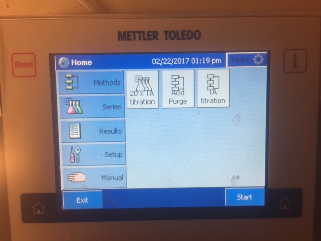
• After your sample is loaded, go back to the titrator screen and select "TA Titration"

• Pressing that brings up a setup screen where we need to input a sample name, and a sample weight. First click the right side of the ID 1 box.

• Type in the name you'd like the sample to have and select OK.

• That updates the Sample ID, next click the right side of the Weight box and input the weight you recorded earlier

• Once you've done that, you should be ready to go and press "Start" at the bottom.

• Two errors will pop up, both associated with the pH probe age. Just click ok.

• The titrator will begin by aerating the sample for 10 seconds, to ensure the sample is well mixed prior to adding acid.

• The titrator then takes an initial reading, which may be higher than expected due to the time it takes for the sample to equilibrate with the liquid already in the pH probe.

• The titrator then begins adding acid in 0.1 mL increments until the voltage reading from the sample is 200 mV. This should take ~ 2.0 - 2.2 mL of acid. After the sample reaches 200 mV, the titrator aerates the sample, without any additional acid being added for 6 minutes to offers any left over CO2. After the aerations step, the machine adds acid in 0.05 mL increments, until it reaches an end point of 250 mV, which is equivalent to a pH of 3.0.

• The run is complete when the screen shows this. It should take ~ 15-16 minutes per sample. Hit ok. We're now done with the titrator, and we move over to the laptop.

• Click the Reports tab on the left hand side of the screen. You may need to click both the Last 24 Hour and Last 3 Day buttons for the application to update with your newest readings.

• Click the report you're interested in, likely the one on top as that will be the newest

• Hit Export in the upper right hand corner, then Export To:, and select CSV file.

• Hit ok, these are just character encoding options for the csv file.

• Name the file and select where you'd like it to save.

• Transfer the csv file to a computer of your choice, or run the local R script Micah wrote to calculate TA from the csv file. In the line of the script you have to supply C, the concentration of the acid, located on the bottle and S, the salinity of the sample, for the CRM supplied by the UCSD CRM information site linked above.

• The script outputs a single number, a TA value. Our goal was ~2232, so we were close, but not within that 10 range we'd like.

• Run 2-3 CRM samples. Ideally, the CRM samples would all be +/- 10 units from the UCSD published standard, but if not, there is the option of taking the difference from the mean of your CRM samples from the published standard, and using that as an offset for your unknowns.

• After you feel comfortable that the CRMs are reading properly, proceed with unknown samples following the same protocol. Re-run CRMs every 5-6 unknowns, to ensure there's no probe drift or anything else odd.