Collapsed

Bayesian Hidden Markov Models and their Mixtures for Python

Author

tllake: thom.l.lake@gmail.com

Overview

collapsed is a Python package for working with Hidden Markov Models (HMMs) and Mixtures of HMMs. The focus is on fast implementations of algorithms for inference and learning with reasonably painless extensibility. When these two goals are in conflict, collapsed sacrifices extensibility for speed.

It should be noted that although collapsed takes a Bayesian approach to most things (all parameters have a prior), the library in general assumes you want to produce a point estimate of model parameters. What can I say, I like to consider myself neither a Bayesian or a Frequentist, but an Empiricist. Sometimes we just don't have time to do fully Bayesian posterior inference at test time.

Dependencies

• python
• numpy
• scipy

Models

Currently collapsed supports first order HMMs with compound Gaussian Normal Inverse Wishart, Categorical Dirichlet, or Multivariate Categorical Dirichlet emission distributions, although adding support for user defined emissions is relatively easy. collapsed also allows one to form Finite or Dirichlet Process [Rasmussen1999] mixtures of HMMs.

Learning

collapsed supports a relatively unique set on methods for parameter estimation. In particular collapsed supports learning via

• Collapsed Block Gibbs Sampling [Johnson2008].
• Hard EM/Viterbi [Allahverdyan2011].

Currently there is no support for typical EM/Baum-Welch parameter estimation, although this may be added at some future date. The reason for this omission is twofold.

1.) There are many other implementations of standard EM for HMMs out there. If you really need normal EM, you shouldn't have problems finding an implementation.

2.) In general these two methods are rather versatile and cover a broad class of use cases. If you need really fast training that yields competitive results, use Hard EM. It is at least 2x faster than normal EM (no backward smoothing), and has been found to often perform similarly or better than normal EM, especially in the unsupervised setting [Spitkovsky2010]. If you want a more global search over parameters, don't want to worry about initialization and random restarts, or are just more comfortable with a Bayesian approach, use the block collapsed Gibbs sampling.

Usage

As an example we'll use the classic trick coin. There are two coins. One is fair and the other always comes up tails (we'll represent heads and tails by 0 and 1 respectively). Let's build a trick coin and sample a sequence of outcomes.

import collapsed

n_states, n_symbols = 2, 2
pi = [1.0, 0.0]
A = [[0.95, 0.05], 
     [0.05, 0.95]]
B = [[0.5, 0.5], 
     [0.0, 1.0]]
latent = collapsed.MarkovChain(n_states, pi, A)
observed = collapsed.DirCat(n_states, n_symbols, B)
trick_coin = collapsed.HMM(latent, observed)
y_true, x = trick_coin.generate_sample(150)

Now let's build a model with uniform Dirichlet priors over all the parameters, and try to infer what coin was used at what time.

a_pi = [1.0, 1.0]
a_A = [[1.0, 1.0],
       [1.0, 1.0]]
a_B = [[1.0, 1.0],
       [1.0, 1.0]] 
latent = collapsed.MarkovChain(n_states, a_pi, a_A) 
observed = collapsed.DirCat(n_states, n_symbols, a_B)
model = collapsed.HMM(latent, observed)

At this point things might seem a little fishy. pi, A, B are the initial, transition and emission parameters respectively, while a_pi, a_A, a_B are hyper-parameters, so why is the usage the same? In short, because collapsed works with compound distributions, the difference between actual observations and hyper-parameters gets blurry.

In fact what we passed to collapsed.HMM in both cases were hyper-parameters. It just so happens that since we haven't added any data to trick_coin, things work the way we want. When calling trick_coin.generate_sample, the trick_coin object calculates the expected value of the parameters given the observed data. Having not observed any data, these coincide exactly to the hyper-parameters we passed in, and life is good. We could have got the same parameters using any scaled version of what we used above, for example A = [[95., 5.], [5., 95]].

Moving on, next we need to add our data to model. Since we're assuming we don't have any information about the latent state sequence that generated x, we'll initialize it randomly by proposing a latent state sequence from our model. We'll then run Gibbs sampling on our model for 150 iterations.

score, y = model.propose(x)
model.add_data(y, x)
model.gibbs(150)

Let's see if we can tell the difference between a draw from a fair coin, and the two state trick_coin.

import numpy as np
x1 = np.random.randint(0, 2, 50)
_, x2 = trick_coin.generate_sample(50)
print model.likelihood(x1)
# Out: -38.3722907758
print model.likelihood(x2)
# Out: -25.0656733858

Great, that works! Recovering the true latent states is more difficult, but collapsed does a reasonable job. We can do this two ways. First, we can use the state of the sampler at the final iteration. collapsed.HMM stores all the data in the order we added it as (latent, observed) tuples in a list aptly named data, so all we need to do is index into it. We ignore the observation because we don't need it.

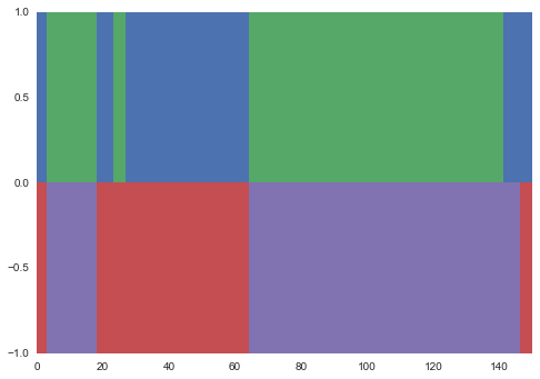
y_sample, _ = model.data[0]

The alternative is to use the expected value of the parameters to infer the maximum a posteriori (MAP) state sequence. We'll plot this against the actual latent state sequence.

import matplotlib.pyplot as plt
import seaborn as sns # seaborn is awesome, you should use it.
score, y_pred = model.map(x)
pal = sns.color_palette()
for t in range(len(y_true)):
    plt.bar(t, 1, width=1, linewidth=0, color=pal[y_true[t]])
    plt.bar(t, -1, width=1, linewidth=0, color=pal[y_pred[t] + 2])

I get something like the following, which looks pretty good.

References

@inproceedings{Rasmussen1999,
  title={The infinite Gaussian mixture model.},
  author={Rasmussen, Carl Edward},
  booktitle={NIPS},
  volume={12},
  pages={554--560},
  year={1999}
}

@inproceedings{Johnson2008,
  title={A comparison of Bayesian estimators for unsupervised Hidden Markov Model POS taggers},
  author={Gao, Jianfeng and Johnson, Mark},
  booktitle={Proceedings of the Conference on Empirical Methods in Natural Language Processing},
  pages={344--352},
  year={2008},
  organization={Association for Computational Linguistics}
}

@inproceedings{Allahverdyan2011,
  title={Comparative analysis of Viterbi training and maximum likelihood estimation for HMMs},
  author={Allahverdyan, Armen and Galstyan, Aram},
  booktitle={Advances in Neural Information Processing Systems},
  pages={1674--1682},
  year={2011}
}

@inproceedings{Spitkovsky2010,
  title={Viterbi training improves unsupervised dependency parsing},
  author={Spitkovsky, Valentin I and Alshawi, Hiyan and Jurafsky, Daniel and Manning, Christopher D},
  booktitle={Proceedings of the Fourteenth Conference on Computational Natural Language Learning},
  pages={9--17},
  year={2010},
  organization={Association for Computational Linguistics}
}